Category Archives: VBA

Average with NULL values

You have a sales report. Each sales rep from A to J have sold a number of products except D and H.

We should count the average sales.

The standard average formula counts only numbers. For example, sales reps D and H are not included. Sum of numbers is 447. If you divide that with eight, that is roughly 56.

When sales reps D and H are on the payroll, they need to be included in the average counting. 56 is too high average as two sales reps have zero sales.

Data includes NULL values.

The more realistic average is around 45.

To make denominator as ten, we have few options available.

We can count cell with value in B1:B10 and then add cells without value B1:B10 to include all the cells. Also ROWS function counts rows in data range.

We count the sum in B1:B10 and then we divide by COUNT + COUNTBLANK or by ROWS -function. Then we have the wanted 45 as a result.

Another option is to populate NULL values with zero numbers, then standard average can be used.

Activate the B1:B10 range and execute the macro below.

Sub z_zero()

Dim cell As Range

For Each cell In Selection

If cell.Value = vbNullString Then

    cell.Value = 0

End If

Next cell

End Sub

NULL values are in Excel VBA called as vbNullString. If the macro finds NULL value in the range, then that is replaced by zero. If the value is zero, then it is NULL.

Activate the values, then execute the macro. Now NULL values have been replaced by zero, and standard AVERAGE behaves as we want.

We can count average in Access too.

The same values are in Access.

A query was created.

The SQL is:

SELECT Avg(IIf(IsNull(sal),0,sal)) AS Expr1

FROM tab;

The result is the same as in Excel.

We have nested formulas AVG, IIF and ISNULL. In other SQL dialects same thing can be done with AVG and IFNULL.

SQL sentence is short compared to do same in Excel. Excel is a better tool number crunching, but if you can do something with SQL, Access is worth trying out.  
INT function

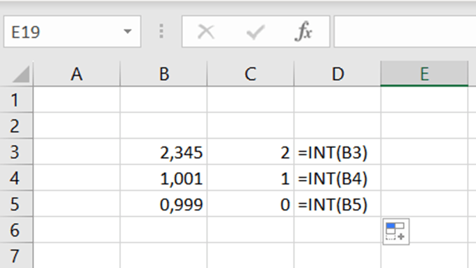
Do you know INT function ? It returns the integer or whole number.

This is not so complex.

In a park place, parking is free for the first two hours, after that parking costs two euros per beginning hour. Two hours and one minute parking costs two euros, two hours and 59 minutes costs two euros.

How to count this in Excel ?

The sentence is: =IF(B2<2;0;IF(B2-2>INT(B2-2);INT(B2-2)*2+2;(B2-2)*2))

If parking takes less than two hours, the fee is zero.

If the value minus two is higher than integer, meaning that there are decimals, then IF takes the integer value minus two and multiplies by two and adds two. If the value is not higher than integer, then value minus two is multiplied by two.

If we have value 4,1 – 2, that is higher than INT(4,1-2) which is two. Then we take integer (4-2) that is two multiplied by two and finally add two. That is six. If the value is sharp four, then just multiply four minus two by two, that is four.

If someone enters a negative value, the sentence returns zero. The input value is less than 2. Parking time cannot be negative but sentence was tested this way.

In case you prefer own functions, the respective code is here:

Function z_park2(hrs)

If hrs < 2 Then

    z_park2 = 0

ElseIf (hrs – 2) > Int(hrs – 2) Then

    z_park2 = Int(hrs – 2) * 2 + 2

Else

    z_park2 = (hrs – 2) * 2

End If

End Function

The function returns the z_park2 value, which counted with input value hrs. If hrs is less than two, then z_part value is zero. If input value minus two is higher than integer for hrs minus two, then integer for input value minus two is multiplied by two and add two. If input value minus two is same as integer value minus two , meaning there is no decimals, then input value minus two is multiplied by two.

INT function in Visual Basic is similar than in Excel.

The input value needs to be in decimal format. Unfortunately, hh:mm format does not yet work.

As I started with, INT is not so complex function. Still, it nice to find how to use even simple functions. On the other hand, it is nice to make Excel count something which you could count mentally.

VLOOKUP and TRIM

You have a simple VLOOKUP, but somehow it does not work. Even though VLOOKUP is correctly written. This might depend on several things.

VLOOKUP is looking for qw34 value in the range (B3:C5). Then one column right from qw34 is selected. The expected value is 1, but the VLOOKUP does not return that value.

As said, this might depend on several things. In our case, there are invisible spaces after qw34 in the cell of B3. This can be found with LEN function. LEN return the number of characters in a string, invisible spaces are counted and increasing the length.

The VLOOKUP does not return 1 as the value in B3 is “qw34  ” with six characters and the value in F3 is “qw34” with four characters. VLOOKUP does not simply find “qw34” in B3:B5.

We can correct with TRIM function, which is removing spaces.

To do this easiest way, we can execute Visual Basic code to manipulate the cells with TRIM.

Sub z_vlookup_trim()

Dim za, zn

Do

    za = ActiveCell.Value

    zn = Application.WorksheetFunction.Trim(za)

    ActiveCell.Value = zn

    ActiveCell.Offset(1, 0).Select

Loop Until ActiveCell = “”

End Sub

First, the variables za and zn are introduced. The variable za is receiving the value from the active cell. If you execute the macro when the cell B3 is activated, then za gets the value “qw34  ”. The variable zn is za manipulated with Excel function TRIM. The value for zn is “qw34”. The VBA proceeds downwards till the active cell is empty.

Place the cursor in B3 and execute the macro.

After the macro has been executed, the TRIM has trimmed the B3:B5 area from spaces. VLOOKUP in G3 finds the value one. One benefit using a macro is that we don’t have to add any new values in a worksheet.

The expression Application.WorksheetFunction. is a useful way to call an Excel function inside VBA macro.

Running number

You have list of items in Excel like different fruits. You would like to add a running number in front of the items.

You have:

Apple

Orange

Pear

Pineapple

But you would like to have:

1. Apple

2. Orange

3. Pear

4. Pineapple

The list should start with a running number.

The starting point is this.

You can do like this. Just copy and paste as values cells E3:E6. Then delete the cells B2:C6. The result is neat but requires some manual work.

We can have a VBA for this, too.

Sub z_runnum()

Dim zn

Dim za

zn = 1

Do Until ActiveCell = “”

    za = ActiveCell.Value

    ActiveCell.Value = zn & “. ” & za

    ActiveCell.Offset(1, 0).Select

    zn = zn + 1

Loop

End Sub

The VBA is even pretty short. Variable zn is the running number which starts from the one. If you would like to start with zero just set zn to zero, ZN = 0. Za is the value of the cell to be investigated. The VBA is looping till it hits an empty cell.

The value of the active cell is captured into variable za. The new content of the cell is running number zn, dot, space and the original value of the cell ZA.

Just place the cursor on the first cell value and execute VBA.

This is the result.

The benefits of VBA are that you don’t have to clean the data afterwards. It is fast and effective especially if you have large amounts of data.

Dynamic SUM for data range

You have a range of cells with values. Then you want to create sum function at the bottom and on the right hand side of the range.

Sum functions are needed in row 6 and column F. This is easy and can be done manually, of course. Just copy the sum to remaining rows and columns.

If you need to do this process repeatedly, a macro might help you. The VBA is added at the end of this blog.

To run the macro, you need to place the cursor in the top left corner of the data range. In our case, the start cell is B2.

Zs is the address of the start cell, eg B2. Then we go at the end of the B row, the address of that cell is stored in zl. Then we go one line down and add the sum sentence SUM(start cell:end cell), then we go one row upwards and one column to right. If that cell is empty then we need to add the sum sentences for each row. If that cell is not empty then we continue counting column sums.

After counting column sums, then we go to the start cell, in this case B2. Zs and zl are populated again. We move to the right end of the data range. Then we move one step to right and there the SUM(start cell:end cell) sentence will be created. Then we move one row down and one column to left. If the cell is empty, then the macro is finished. If the cell is not empty, then we continue counting row sums.

Instead of manually creating sum sentences, place the cursor in B2 and execute the VBA below.

Sub z_sum2()

Dim zs, zl, zss

zss = ActiveCell.Address

Do

zs = ActiveCell.Address

Selection.End(xlDown).Select

zl = ActiveCell.Address

ActiveCell.Offset(1, 0).Select

ActiveCell.Formula = “=sum(” & zs & “:” & zl & “)”

ActiveCell.Offset(-1, 1).Select

If ActiveCell.Value = “” Then

    GoTo zrow

Else

    Selection.End(xlUp).Select

End If

Loop

zrow:

Range(zss).Select

Do

zs = ActiveCell.Address

Selection.End(xlToRight).Select

zl = ActiveCell.Address

ActiveCell.Offset(0, 1).Select

ActiveCell.Formula = “=sum(” & zs & “:” & zl & “)”

ActiveCell.Offset(1, -1).Select

If ActiveCell.Value = “” Then

    Range(zss).Select

    MsgBox “Done.”

    End

Else

    Selection.End(xlToLeft).Select

End If

Loop

End Sub

Search and count

You have a data range and you should find how many times certain character exists within the data area.

This can be done easily with COUNTIF as follows.

The data range.

Copy the range and select data – data tools – remove duplicates.

Press ok.

The list of 12 values was shortened to 4.

The data range includes unique values D, C, A  and B.

The arguments for COUNTIF are the range where the value is searched and the value which is searched for.

However, if you want to just fast get a number how many times A appears in the data range, we can tackle that with VBA below.

Sub z_count()

Dim cell As Range

Dim arv, cnt

arv = InputBox(“Search term”)

cnt = 0

For Each cell In Selection

If cell.Value = arv Then

cnt = cnt + 1

End If

Next cell

MsgBox arv & “:” & cnt, vbOKOnly, “Search macro”

End Sub

The range selection consists of cell variables. Arv is the value to be searched for. Cnt is the counted value of arv. The data range is browsed through and every time arv is found, that is increasing the value of cnt by one. At the end, the cnt is printed in message box.

Activate the data range and execute the macro.

Select the value to be searched for.

The result is the same with COUNTIF. If you want to list all the values, the COUNTIF is practical. In case you repeat this process many times a day and you just want to get the value, VBA might be the worth of trying.

Adding a leading number

You have a long list of receipts written down in Excel. The receipts should be numbered. The first one should be 1. Receipt A, second 2. Receipt B and so forth.

This might be the case when you have receipts as hard copies and you need to number the hard copies. Also the Excel numbering must be in sync with numbers in hard copies.

Of course, you can add a column with running number and the combine the two columns.

This is fine, too. Still, you need to create more columns and in real life cases columns F and G might already have been populated.

Another option is to execute the macro below. Place the cursor where the data begins, in D2.

Sub znum()

Dim num

Dim cv

num = 1

Do Until ActiveCell.Value = “”

cv = ActiveCell.Value

ActiveCell.Value = num & “. ” & cv

ActiveCell.Offset(1, 0).Select

num = num + 1

Loop

End Sub

Variable num is increasing by one after every cell. The variable is added in front of the cell context. The cell context is the variable cv. The macro manipulates the cell one by one and stepping down after each cell. When the next empty cell is found, then the macro ends. You cannot have empty lines within the data.

The benefit of the macro is that it is overriding the existing values in D-columns.

Place the cursor in D2 and execute the macro. This is the result.

Annual growth rate

You bought a flat in 2010 for 130 k€ and sold it in 2020 for 185 k€. How many percent the value of the flat grew annually ?

The formula is ((start value /finish value)^(1/ start year/finish year))-1

This calculation is counting only full years, and calculation gives you a directional value. The idea is not to calculate exact value, but rather to give you an idea about magnitude.

The same value can be counted with own formula, if you feel that more convenient. The functions returns you a short message, if the function finds an error.

Function z_annual2(start_value, finish_value, start_year, finish_year)

On Error GoTo Fehler

z_annual2 = (finish_value / start_value) ^ (1 / (finish_year – start_year)) – 1

z_annual2 = Format(z_annual2, “0.00 %”)

Exit Function

Fehler:

z_annual2 = “Check your input”

End Function

Weekday from WEEKDAY function

When you use WEEKDAY function in Excel, you enter a date like 1.1.2020 and maybe hope to see the weekday. However, WEEKDAY returns you a number. With Return_type argument, you can define the number, but number is still a number. It would be nice to have a weekday like Monday or Tuesday instead of the number.


I have seen some ways to have a weekday instead of number.

I like an IF-sentence.

=IF(WEEKDAY(A4)=1;”Sunday”;IF(WEEKDAY(A4)=2;”Monday”;IF(WEEKDAY(A4)=3;”Tuesday”;IF(WEEKDAY(A4)=4;”Wednesday”;IF(WEEKDAY(A4)=5;”Thursday”;IF(WEEKDAY(A4)=6;”Friday”;IF(WEEKDAY(A4)=7;”Saturday”)))))))

It is a bit long, but once I wrote it, you can just copy paste it.

Just paste the text to cell B4.

Another option is that you create your own function with the same logic.

Function z_wd(z_d As Date)

If WorksheetFunction.Weekday(z_d) = 1 Then

    z_wd = “Sunday”

ElseIf WorksheetFunction.Weekday(z_d) = 2 Then

    z_wd = “Monday”

ElseIf WorksheetFunction.Weekday(z_d) = 3 Then

    z_wd = “Tuesday”

ElseIf WorksheetFunction.Weekday(z_d) = 4 Then

    z_wd = “Wednesday”

ElseIf WorksheetFunction.Weekday(z_d) = 5 Then

    z_wd = “Thursday”

ElseIf WorksheetFunction.Weekday(z_d) = 6 Then

    z_wd = “Friday”

ElseIf WorksheetFunction.Weekday(z_d) = 7 Then

    z_wd = “Saturday”

End If

End Function

To use the function in B2 might be easier than direct IF-sentence.

Increasing values by one

You have a list of values in Excel. All the values which are not empty should be increased by one.

1

1

1

2

Should be

2

2

2

3

You can fill the new values in the cell next to the values with IF-function =IF(B2>0;(B2+1);””) .The correct values are populated next to the original values.

If you don’t want to have an additional column, but original values should be overwritten by new values, you can also execute the macro below.

sub z_plus_one2()

Dim cell As Range

For Each cell In selection

If cell.value > 0 then

cell.Value = cell.value +1

end if

Next cell

End sub

Activate the values and execute the macro.

Counting basic net salary

If you want to calculate fast and simply how much would somebody’s net salary be, then you might want to use the macro below.

Gross salary is deducted with following payments

Income tax: this is from employee’s tax card

Employee’s part for work pension: 7,15 % of gross salary in case the employee is 17-52 or 63-67 of age.

Employee’s part for unemployment insurance: 1,25 % of gross salary in case the employee is 17-64 of age.

This can be done easily by writing the formulas manually. However, if you do this repeatedly, sooner or later you will value a macro.


Fill the cells with yellow filling: gross salary and income tax percentage.

This model does not take into consideration taxable benefits like mobile phone or taxable bonuses on top of basic salary.

Sub z_payroll_basic_macro()

Application.ScreenUpdating = False

ActiveCell.FormulaR1C1 = "Gross"
ActiveCell.Offset(1, 0).Range("A1").Select
ActiveCell.FormulaR1C1 = "Tax"
ActiveCell.Offset(1, 0).Range("A1").Select
ActiveCell.FormulaR1C1 = "Pension"
ActiveCell.Offset(1, 0).Range("A1").Select
ActiveCell.FormulaR1C1 = "Unempl"
ActiveCell.Offset(-2, 2).Range("A1:A3").Select

Selection.NumberFormat = "0.00%"
ActiveCell.Offset(1, 0).Range("A1").Select
ActiveCell.FormulaR1C1 = "7.15%"
ActiveCell.Offset(1, 0).Range("A1").Select
ActiveCell.FormulaR1C1 = "1.25%"
ActiveCell.Offset(-2, -1).Range("A1").Select
ActiveCell.FormulaR1C1 = "=ROUND(R[-1]C*RC[1], 2)"
ActiveCell.Offset(1, 0).Select
ActiveCell.FormulaR1C1 = "=ROUND(R[-2]C*RC[1], 2)"
ActiveCell.Offset(1, 0).Select
ActiveCell.FormulaR1C1 = "=ROUND(R[-3]C*RC[1], 2)"
ActiveCell.Offset(1, 0).Select


ActiveCell.FormulaR1C1 = "=R[-4]C-SUM(R[-3]C:R[-1]C)"
ActiveCell.Offset(0, -1).Range("A1").Select
ActiveCell.FormulaR1C1 = "netto"
ActiveCell.Offset(-4, 0).Range("A1").Select

    ActiveCell.Offset(0, 1).Range("A1").Select
    With Selection.Interior
        .Pattern = xlSolid
        .PatternColorIndex = xlAutomatic
        .Color = 65535
        .TintAndShade = 0
        .PatternTintAndShade = 0
    End With
    ActiveCell.Offset(1, 1).Range("A1").Select
    With Selection.Interior
        .Pattern = xlSolid
        .PatternColorIndex = xlAutomatic
        .Color = 65535
        .TintAndShade = 0
        .PatternTintAndShade = 0
    End With

Application.ScreenUpdating = True
End Sub


I did not write this macro manually, but recorded two macros and modified them.

Screen updates have been turned off, that the screen does not flash, when the macro is executed. You can remove the code lines, if you want. In case you want the screen updates to be disabled in some other macros, you can copy the lines here and add them to another macro.

This blog has been published earlier but now updated according to the year 2020 percentages.

Every second A every second B

Values are downloaded to Excel. Dimension for the first row is A and second B and so on. Parameter for the first value is A, second is B and so on. When downloading the data, the parameter is missing and should be added manually.

The starting point.

The end result. This should be done.

This can be done in many ways.

Write manually A and B in A3 and in A4. Activate cells A3 and A4. Touch with cursor the square in low right hand corner in A4 and double click.

Sub Z_AB

ActiveCell.Value = “A”

ActiveCell.Offset(1, 0).Select

ActiveCell.Value = “B”

ActiveCell.Offset(1, 0).Select

End sub

This macro is creating one pair of A and B. If you assign the macro to shortcut key and just press the key as many times as needed.

If you know that there are 20000 records of data and 10000 pairs of A and B should be added, you can use the macro below.

Sub Z_AB2

Dim c

For c = 1 to 10000

ActiveCell.Value = “A”

ActiveCell.Offset(1, 0).Select

ActiveCell.Value = “B”

ActiveCell.Offset(1, 0).Select

Next c

End sub

The macros are useful, if a zero value is presented as blank cell. The double clicking does not work.

Decimal symbol and thousands separator

For me it has happened many times, that decimal separator is incorrect.

Comma is thousand separator and dot decimal separator. For me, the thousand separator is not needed and decimal separator should be comma. This is my view, someone might disagree.

First, check the number formatting settings in operating system and in Excel.

Take control panel, and number formats under clock and region header.

Select additional settings.

You will find here decimal separator (decimal symbol).

In Excel:

In Excel decimal and thousand separators are in file – options – advanced page.

If “use system separator” is unticked, then

Excel understands 1,500 to be 1500.

When “use system separator” is ticked, then

Excel calculates correctly, to my purposes.

Check the number formatting for the cell by home – number – format cells. Shortcut to this transaction is control + 1.

One option is to manually remove first the comma and the replace dot with comma. You can do this control + F and then control + H.

You can also record macro, and play the macro whenever needed. Here is the recorded VBA. I did not write this VBA, but simply recorded the macro and captured VBA.

Sub Z_commadot ()

    Selection.Replace What:=”,”, Replacement:=””, LookAt:=xlPart, _

        SearchOrder:=xlByRows, MatchCase:=False, SearchFormat:=False, _

        ReplaceFormat:=False

    Selection.Replace What:=”.”, Replacement:=”,”, LookAt:=xlPart, _

        SearchOrder:=xlByRows, MatchCase:=False, SearchFormat:=False, _

        ReplaceFormat:=False

‘         data – text to columns part

        Selection.TextToColumns Destination:=ActiveCell, DataType:=xlDelimited, _

        TextQualifier:=xlDoubleQuote, ConsecutiveDelimiter:=False, Tab:=True, _

        Semicolon:=False, Comma:=False, Space:=False, Other:=False, FieldInfo _

        :=Array(1, 1), TrailingMinusNumbers:=True

End Sub

A cell value in a message box

You have a very large Excel sheet. At the end of rows and columns are SUM formulas.

Cell AO42 contain the total sum.

Whenever you change any cell within range, the value in AO42 will change. To see the value in AP42, you should each time to scroll right and down to see the value.

You change the cell value in H8, but you would like to know immediately how much is the grand total in AO42. One option is to scroll down right to AO42. If you need to constantly fine tune numbers, it is time consuming to scroll right and down after each change.

However, if you have a macro to bring the value in message box.

Like this. When you assign a shortcut key to macro, you can check the grand total by pressing shortcut key.

VBA:

Sub z_tot()

Dim tul

On Error GoTo Fehler

tul = Round(Range(“ao42”).Value, 2)

MsgBox “The total sum is: ” & tul & “.”, _

vbOKOnly, “Own macro”

Exit Sub

Fehler:

    MsgBox “Error somewhere.”, vbOKOnly, ” Own macro”

    Exit Sub

End Sub

On error statement tracks whether the cell does not contain any reasonable value. If the function in AO42 does not return any value, the ROUND cannot round and VBA hits an error. With on error, the macro just brings a message box.

In case you want to see the row or column total instead of the grand total, you should scroll downwards or to right to see the row or the column total.

The macros below return the row and column totals based on the active cell. The active cell means the cell where the cursor is. If you have changed a cell and you would like to track the column or row total, do not select another cell, but keep the cursor in the cell where you made the change.

Sub z_col_tot()

Dim tul

Dim zr

Dim zv

Dim zs

zs = ActiveCell.Address

zr = ActiveCell.Row

ActiveCell.Offset((42 – zr), 0).Select

zv = ActiveCell.Address

Range(zs).Select

On Error GoTo Fehler

tul = Round(Range(zv).Value, 2)

MsgBox “The total sum for column is: ” & tul & “.”, _

vbOKOnly, “Own macro”

Exit Sub

Fehler:

    MsgBox “Error somewhere.”, vbOKOnly, ” Own macro”

    Exit Sub

End Sub

To see the row total

Sub z_row_tot()

Dim tul

Dim zc

Dim zv

Dim zs

zs = ActiveCell.Address

zc = ActiveCell.Column

ActiveCell.Offset(0, (41 – zc)).Select

zv = ActiveCell.Address

Range(zs).Select

On Error GoTo Fehler

tul = Round(Range(zv).Value, 2)

MsgBox “The total sum for row is: ” & tul & “.”, _

vbOKOnly, “Own macro”

Exit Sub

Fehler:

    MsgBox “Error somewhere.”, vbOKOnly, ” Own macro”

    Exit Sub

End Sub

Searching for two terms

Years ago I was asked, if it is possible to search with two search criterias in worksheet. So, I want to search both A and B whichever I find first. Normally you search in Excel with just one criteria like this:

To find take home-find & select – find.

First search for A.

Then search for B.

If you however want to search for both A and B at the same go, then we need some further development.

Here is the VBA code from a recorded macro searching for A.

Sub Z_search()

‘ Z_search Macro


Cells.Find(What:=”A”, After:=ActiveCell, LookIn:=xlFormulas, LookAt:= _
xlPart, SearchOrder:=xlByRows, SearchDirection:=xlNext, MatchCase:=False _
, SearchFormat:=False).Activate
End Sub

To modify the VBA, first the main block should be doubled that first the search term 1 is searched and the search term 2. Static “A” should be replaced by parameter. The main block is copied from recorded macro.

On Error Resume Next means that if VBA hits an error, the code is not stopped there. This is needed because if the macro does not find anything, it will face a run time error 91. With this line the VBA does not stop with run time error.

Here is the code

Sub z_search()

‘ z_search Macro

Dim s1, s2
s1 = InputBox(“1st search term”)
s2 = InputBox(“2nd search term”)

On Error Resume Next

‘ this part was recorded and then what-parameter was modified, I did not write this myself

Cells.Find(What:=s1, After:=ActiveCell, LookIn:=xlFormulas, LookAt:= _
xlPart, SearchOrder:=xlByRows, SearchDirection:=xlNext, MatchCase:=False _
, SearchFormat:=False).Activate

Cells.Find(What:=s2, After:=ActiveCell, LookIn:=xlFormulas, LookAt:= _
xlPart, SearchOrder:=xlByRows, SearchDirection:=xlNext, MatchCase:=False _
, SearchFormat:=False).Activate

End Sub

If the code find both the first term and the second term, then the program is showing the place of the second term, but this is a functionality.

Counting total debit or credit with SUM and SUMIF

You have list of accounting postings. For some reason, you need to check that sum of debit postings equals to sum of credit postings. There might be an error in closing process, and you just want to double check in Excel that no mismatch has taken place in accounting. System should not allow a posting when debit differs from credit, but this is a case to really make sure that no mismatch exists.

Accounting data was simplified. Imagine, that you have hundreds of accounts and thousands of postings.

One simply option is to count with SUMIF. First, you need to count sum for every column like in row 10. Totals for debit and credit are counted with SUMIF. In SUMIF you need to first determine range for Ds and Cs that is B2:M2. Then criteria is needed whether it is D or C, B13 or B14. Finally you enter sum range B10:M10. If in row 2 the value equals to B13 or B14 then sum is counted from row 10. This works, but is you have lots of data, this might be bit difficult as you need to count each column sum separately.

Another bit easier solution is to count with SUMIF without interim SUMs. Write following formula =SUM(IF(B2:M2=B11;B3:M8)) in C11 and press control+shift+enter. The result should be {=SUM(IF(B2:M2=B12;B3:M8))}, but don’t write that, that is the outcome after control+shift+enter.

SUM is counted in M3:M8 if values in B2:M2 equals to B11. Don’t forget control+shift+enter.

Third option is to use column numbering.

COLUMN function is turning column letter to number.

In our case debits are in paired columns and credits in impaired.

Paired and impaired numbers can be traced by MOD function.

If MOD is 1 then the column is for debits and 0 for credits.

Row 10 includes sum of each row like M10 sums M3:M8. Row 9 determines whether the column number is paired or impaired. SUMIF in C12 is a normal SUMIF. First you need to feed the range meaning Ds and Cs, then criteria C or D is needed, last sum range is given.

Fourth option is based on paired and impaired column numbers. A custom made formula is summing up the values in paired or impaired columns. For paired cells dc parameter is 0 and impaired 1. Then activate the sum area. That’s all.

The custom made function:

Function z_dc(dc, rng As Range)

Dim cell As Range

Dim para

If dc = 0 Then

    para = 0

ElseIf dc = 1 Then

    para = 1

End If

z_dc = 0

For Each cell In rng

If (cell.Column) Mod 2 = para Then

    z_dc = (z_dc + cell.Value)

End If

Next cell

End Function

Dynamic SUM function

Lists of data is downloaded vertically to Excel. Lists consist of different amount of numbers. At the end of each list, sum should be calculated.

B, D, F and H columns should be summed separately. Meaning, Cell B20 should sum values B2:B19, D9 sums D2:D8 and so on.

This can be done manually, of course. However, a macro can be built to make process bit faster.

The VBA is short and neat.

Sub z_dyn()

Dim zs, zl

zs = ActiveCell.Address

Selection.End(xlDown).Select

zl = ActiveCell.Address

ActiveCell.Offset(1, 0).Select

ActiveCell.Formula = “=sum(” & zs & “:” & zl & “)”

End Sub

Activate the first cell of list, like B2, and execute the macro.

Zs and zl are variables for the start cell and the last cell. The activated cell, when the macro is executed, is the first cell of list, like B2. After that the macro jumps till the last cell of list, like B19. Then macro takes one step down and populates the cell with the sum function sum(first cell:last cell).

Activate the cell B2 and execute the macro. The result is here.

In case you want to calculate the AVERAGE of each list, just change SUM to average in VBA.

Self made functions

If you repeat same calculation many times, it is useful to create your own function. As macro is repeating predefined steps, function returns a value.

Capital asset pricing model: expected return equals to risk free rate + (expected return of market portfolio – risk free rate) times beta-factor of the security.

This can be easily calculated in Excel.

Calculating CAPM manually is not an issue, but as said, repeating the same process often takes more time than creating a self made formula.

Function z_ser(fr, mr, b)

z_ser = fr + (mr – fr) * b

End Function

Save the functions in VBA editor under personal workbook, then the formula is available in all your Excel workbooks.

Function is calculating the value for z_ser based on input values rf, mr and b. I used to start my own functions with z_ to sort out my own functions. Another practice is to keep variable names short. It is faster to write and possibility for typing errors is lower than with long names.

Once you are done with VBA and you start to write formula in Excel application side, press fx button

Self made function can be used in the same way as Excel standard functions.

Finding current date

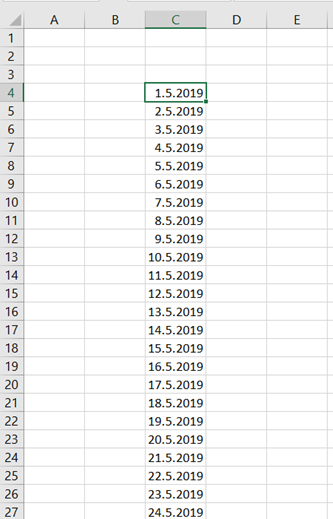
You have list of dates. In case you keep manually a record per each date. You should find the current date from a list of dates.

You have a list of dates. For finding the current date, you can manually browse and stop when you find the correct date. To automate the process, a macro can be created which is checking the correct date.

The formula TODAY is returning the current date. The value is stored in the cell F1.

The macro itself is here:

Sub z_today()

Dim tod As Date

tod = Range(“f1”).Value

Range(“c4”).Select

Do

If ActiveCell.Value = tod Then

    MsgBox “Today is ” & tod & “.”, vbOKOnly, “Own macro”

    End

Else

    ActiveCell.Offset(1, 0).Select

End If

Loop

End Sub

The variable tod is taking the value from the cell F1. The macro activates the cell C4 and compares that to F1. If the value is the same, meaning the cell in C-row holds the current date, then the macro pops up the message box and ends execution. If the current date was not found, then the macro takes on step downwards and compares the values again.

When you execute the macro, the macro finds the current date and you don’t have to visually browse the data area.

Saving Excel workbook with a macro

Several reports are downloaded to Excel one by one. Each report will be saved separately as a file to harddisk.

When the report is completed you can just take file-save as without any macros.

It is possible to make a process faster to have a macro saving the file.


Presuming, you take a report by region and period one by one, the data is pasted to columns A to D, row 1 is a header.

It is useful to find some logic for file naming, that you don’t have to name the files separately manually. In the case above, I have taken region_period_number as naming convention. As the name is populated with links, it makes saving the files bit faster.

The macro looks like this:

Sub Z_SaveDocument()

‘ SaveDoc Macro

Dim FileName

FileName = Range(“g11”).Value

    ActiveWorkbook.SaveAs FileName:=”C:\Excel test\” & FileName & “.xlsm”, _

        FileFormat:=xlOpenXMLWorkbookMacroEnabled, CreateBackup:=False

End Sub

The cell G11 defines the file name. I have created a variable to look the macro nicer. The files will be saved in folder C:\Excel test\. You might want to change the file path fitting your own file structure. The extension for files is .xlsm as the files contain a macro. As said, the file name is a variable. As a static value, the file path would be C:\Excel test\ South_7_1.xlsm.

It is useful to create a button in Excel workbook, then executing the macro is pretty fast. I have not saved this macro to personal workbook as the macro is not needed in every Excel workbooks but only this specific Excel workbook.

Enter the data to range A2:D19 and press the button. Looks like nothing happened but check your C:Excel test folder with file explorer.

Paste the new data to the range and press the button again.

Automating with macro and shortcut key

Most of Excel users have sometimes changed the calculated value to static value, I bet. This is easy.

ISFORMULA formula is checking whether the value is calculated by a formula or a static value.

Number 2 in D3 is a calculated value, ISFORMULA returns the value TRUE. To make it static 2

Activate the cell D3.

Select Copy or press control + C.

Then take paste values and press enter to empty the clipboard.

Now ISFORMULA also finds that it is not calculated anymore.

If you want to do the process above, create a macro.

Take view – macros -record macro. Activate Use relative references.

Store the macro in your personal workbook. Then the macro is available in every Excel workbook. Add also a shortcut key.

Repeat the steps above to copy and paste as values.

After the steps just stop recording.

 Check the VBA code from the developer-visual basic. It should look like this.

Sub Own_name()

    Selection.Copy

    Selection.PasteSpecial Paste:=xlPasteValues

    ActiveSheet.Paste

    Application.CutCopyMode = False

End Sub

Instead of recording macro, you can also copy the code above.

To run macro quickly, you can add a shortcut key. Now even a simple task has been automated with macro. If you repeat copy-paste as values several times a day, like I do, macro with shortcut key will save your time.

IF formula for reporting dimensions

In the report you have two reporting dimensions. Both the dimensions may have values from A to G. If both the dimensions in the same record hold the value F, then this should be notified. In this case, I am not interested in reporting values, like sales volumes, but only in dimensions.

Easier solution is that is Excel just writes a mark next to dimensions.

To define the dimension values I have used RANDBETWEEN function.

=CHAR(RANDBETWEEN(65;71)) is returning a random value between A to G. Of course, you can manually enter any values, but the function is to automate and fasten the process.

In case your reporting dimensions are in C and D columns, the if sentence in cell E3 is

=IF(AND(C3=”F”;D3=”F”);”2F”;””)

IF-sentence checks that both C3 and D3 hold the value F, in this case, the IF-formula returns the value 2F. If C3 and D3 are not Fs, the IF does not return anything.

As a result the third reporting dimension is created with a new dimension value.

If you want that dimensions are changed to something else than original value F, if both the dimensions hold the value F, then we need macro to overwrite F values to eg 2F.

Sub FF2()

Range(“s3”).Select

Do Until ActiveCell = “”

If ActiveCell = “F” Then

ActiveCell.Offset(0, -1).Select

    If ActiveCell = “F” Then

        ActiveCell = “2F”

        ActiveCell.Offset(0, 1).Select

        ActiveCell = “2F”

    Else

        ActiveCell.Offset(0, 1).Select

    End If

End If

    ActiveCell.Offset(1, 0).Select

Loop

End Sub

The program starts with cell S3. This is the first record, the right hand side dimension. Program is executed till the end of the data range, till the program finds the first empty cell. If the program finds “F” in right side column, then the program checks also the left side dimension in the same record. If that is “F” too, then the program changes both F values to 2F values. If only the right side is F but the left not, then this record should not be overwritten. At the end, program has changed F value to 2F, if both the dimensions in the same record are F.

Now no new columns are added to report, but a new dimension value 2F is introduced, if both the dimensions are F in the same record.

Populating empty cells

The report leaves some cells blank, when report is downloaded to Excel. If cell is blank, the cell should have same value as the cell above. Eg. A5 should be 1, and B5 B, A6 should be 1, and B6 B. In order to have data coherent for Pivot, all the cells in the range A4:B25 should be populated.

You can tackle this issue by VBA or by Excel’s own functionality.

Activate the cells A4:B25 and execute the macro below.

Sub Emptycell()
Dim cell As Range
For Each cell In Selection
If cell= “” then
cell. FormulaR1C1 = “=R[-1]C”
end if
Next cell
End Sub

An other way is to use Go to functionality in Excel.

Activate the cells A4:B25.

In Excel select home and in right corner find & select and Go To. Or press control + G.

Press special -button.

Select blanks and press ok

Write equals shift + 0 and press arrow upwards once. This should be the result.

Press control + enter.

After populating the cells, I normally copy and paste as values, so that the values would not be changed anymore.

Delete empty rows in Excel

When downloading data from ERP to Excel, every second row in Excel is populated and every other is blank.

The Excel would look something like this.

Before you execute the macro, write “end” in the A column cell after the data area.

Like this.

The macro is here:

Sub deleteemptyrows()
Range(“a1”).Select

Do Until ActiveCell = “end”
If ActiveCell.Value = “” Then
ActiveCell.Rows(“1:1”).EntireRow.Select
Selection.Delete Shift:=xlUp
Else
ActiveCell.Offset(1, 0).Select
End If

Loop

MsgBox "Macro done", vbOKOnly, "Own macro"

End Sub

The macro takes the cursor to cell A1. Then the macro checks every cell in A column, if the cell is empty then the row is deleted. If the cell is populated, then the macro jumps to the next downwards in A column.

The result should be this: