The countries are ranked in order based on the medals the country has won in races. The best country has won more gold medals than other countries. The countries which did not win any gold medals are ranked based on how many silver medals they got. The countries which did not win any gold or silver medals are listed by the number of their bronze medals.
If country won one gold medal is that country ranked higher than a country which won 10 silver medals but no gold medals.
G, S and B stand for gold, silver and bronze, just for clarification.
We need to create a reference number for all the countries, the reference number depends on the number of medals the country achieved.
The number of gold medals is multiplied by 1000 and number of silver medals by 100. Then number of bronze medals is added.
Country A won nine gold medals, six silver medals and eight gold medals. Therefore, the reference number for the country A is 8 * 1000 + 6 * 100 + 8= 9608.
Then we can rank the countries, so that number one is the best country.
In our case, function RANK.EQ holds just two arguments. Number, which is ranked, and reference numbers to which the number is compared. The third argument, order, is also possible. In this case, it is not needed. If we wanted to rank the last country as one, we would just enter 1 as order.
Finally, we could set up a podium. We mark 1, 2, and 3. Then Excel should look for us to decide which country is the first, second or third.
For that, we need two functions INDEX and MATCH. I will introduce the functions.
For INDEX the area B2:E4 is defined first. Row selection is three, meaning we take the third row in the area, meaning row starting with nine. Column selection two means that we take the second value from that row, that is ten.
We have lookup value in B2 and lookup array from B4 to B8. Match type is zero, we are looking for the exact match, sharp two. The number two is the fourth number is the array.
First, we need to use MATCH function to find out that number one is the third number in I4:I13 array. Then we take the third country from C4:C14.
A company of changing chart of account and the system how the book keeping accounts are numbered. Earlier the accounts consisted of four digits. Now all the accounts will have five digits. An extra zero will be added between the first and second digit. For example, 1320 will be 10320 and 1090 will be 10090. How can we automate the change with Excel ?
=LEFT(B4;1)&$B$2&(RIGHT(B4;(LEN(B4)-1)))
First we need to take one digit from the left with LEFT(B4;1). The with &$B$2& we add the zero from B2. I have taken zero as reference, if the second digits should be something else than zero, then update the B2 cell. The rest RIGHT(B4;(LEN(B4)-1))) takes digits from right. We are taking three digits as the length of account is four digits and we subtracted one. I did not want to define the number of characters for RIGHT function with static three, as now the sentence works also with numbers longer or shorter than four digits.
The result is correct, but you noticed that numbers aligned to left. Therefore, the values are not numbers. If you need to calculate anything, the cell values should be numbers. As values look like numbers, it would be better that cell category is number.
Only NUMBERVALUE function is added, and the results are in numeric value. The results are aligned to right.
Now we have correct account number. Next task is to find account descriptions from the old account numbers and match them with the new account numbers.
This we can do with VLOOKUP. As we know, VLOOKUP consists of four arguments:
Lookup value, which value we are looking for.
Table array, where the value is being looked for
Column index number, as the value was found in most left column, at which column the value is captured.
Range lookup, we are looking for the exact match for lookup value.
The key in our case is that lookup value may be formed with formulas.
The cell E4 holds the value for 10000, that is the new number for 1000 cash account. We need to have the description for the account 1000 to 10000. The cell value of 10000 needs to be converted to lookup value 1000.
NUMBERVALUE(LEFT(E4;1)&RIGHT(B4;LEN(E4)-2))
We need to take one value from left and then from right the length of the cell subtracted by two. The result needs to be converted into number value. That is how we get 1000 from 10000.
In B and C columns we have old accounts and descriptions. In E columns we have accounts with new numbering, an extra zero has been added between 1st and 2nd number. The description from the old accounts is fetched with VLOOKUP to the new account numbers. Now we have the new chart of accounts in use.
Four questions were asked, and I will answer the questions later in this blog post.
What’s the current line efficiency? (total time / min time)
Are any operators underperforming?
What are the leading factors for downtime?
Do any operators struggle with particular types of operator error?
Let’s check the first the data we got.
Line productivity is a fact table about produced batches.
The product table includes product data and is a dimension table. We are dealing with six products.
Downtime factor table is a dimension table about reasons why downtimes happened. The table is a list of factors and ii the factor was an error caused by an operator.
Line downtime is storing the downtimes per each line and what was the downtime factor. The table is a fact table.
The issue with this table is that it is in matrix format, not a pivot table. Before starting analyzing the data, we need to convert the table into pivot format. I have written a blog post about that.
In brief, load the data as data model. In power query, activate the first column from left and press right mouse button, select “unpivot other columns”.
I will paste the value into separate Excel sheet, as it is easier for me to manage values there.
Just control + v in the Excel sheet.
I have changed the column names to be more descriptive. Factor is foreign key for the primary key in factor dimension table.
Then I loaded the data into MS Access, as usual. I changed the names for the tables to start with either D or F depending on whether the table is dimension or fact. Also, spaces were removed from the field names. It is easier for me when there are no spaces in table or field names, then I don’t have to use quotes or single quotes. SQL queries can be used with Access, too.
The data was loaded from Access into Excel data model.
This is the data model. Product dimension table D_prod is joined to line productivity fact table F_lineprod as both the tables hold product information. The relation is one-to-many. One product appears only once in dimension table but may appear several times in fact table. The factor dimension table D_dfactor is joined to down time fact table F_linedown with factor field. Relationship is again one-to-many. The two fact tables are joined with batch number as the number appears once in F_lineprod table. One batch may have several downtimes.
One notification I must make over the data. The last row in F_lineprod table, the batch starts during the previous day and ends following day. As you note, I have rounded the times into full minutes leaving seconds out.
I will adjust the times that the batch takes 2 hours 10 minutes, but during the same day.
What’s the current line efficiency? (total time / min time)
The first question is to calculate line efficiency. I understand this to be down time divided by total time and I consider product as line.
The downtime is calculated by simply sum of min column in F_linedown table. As the values are given in minutes, the result is divided by 60 to get hours.
=sum(F_linedown[Mins])/60
The values are crosschecked in Access as follows:
SELECT
fd.product AS Expr1,
round(Sum(fn.Mins) / 60, 2) AS Expr2
FROM
F_linedown AS fn,
F_lineprod AS fd
WHERE
fn.batch = fd.batch
GROUP BY
fd.product;
The total time and down time are calculated here:
OR-600 has highest downtime ratio. Other product have quite equal ratio. It is depending on the business is one third of production time reasonable level for downtimes.
If efficiency is calculated by total time minus downtime, the efficiency is 64 %. Another topic is whether 64 % is a good or a bad number.
Are any operators underperforming?
Mac has highest downtime ratio, but differences are minor among operators. Charlie, who has lowest downtime ratio, has the highest absolute downtime. This is due to fact, that total times vary between the operators. Charlie’s total time is 36 % higher than Mac’s.
We can doublecheck the total time with Access as follows:
SELECT
fd.operator AS Expr1,
round(Sum(fn.Mins) / 60, 2) AS Expr2
FROM
F_linedown AS fn,
F_lineprod AS fd
WHERE
fn.batch = fd.batch
GROUP BY
fd.operator;
And down time:
SELECT
fd.operator AS Expr1,
round(Sum(fn.Mins) / 60, 2) AS Expr2
FROM
F_linedown AS fn,
F_lineprod AS fd
WHERE
fn.batch = fd.batch
GROUP BY
fd.operator;
What are the leading factors for downtime?
Downtime have been counted simply with:
=sum(F_linedown[Mins])/60
We take minutes from fact table F_linedown and divide by 60 to get hours.
With downtimes we have deviation. The most common factors for downtime are machine adjustment and machine failure. Those represent more than 40 % of all cases. No emergency stops took place. Conveyor belt jam is very uncommon.
The same can be checked with Access:
SELECT
f.factor,
d.Description,
ROUND(Sum(f.Mins) / 60, 2) AS SumOfMins,
ROUND(
SUM(f.mins) / (
SELECT
SUM(mins)
FROM
F_linedown
),
4
)
FROM
F_linedown AS f,
D_dfactors AS d
WHERE
(((f.factor) = [d].[factor]))
GROUP BY
f.factor,
d.Description
ORDER BY
Sum(f.Mins) DESC;
Do any operators struggle with particular types of operator error?
The only formula which I used here is the same as in previous question. Just summing up the minutes of downtime.
Charlie and Dee have various of operator errors. Dennis and Mac have fewer types of operator errors. Machine adjustment is typical error for Dennis and batch change for Mac.
If you want to check out the same issue in SQL, this is the query I used.
SELECT
fd.Operator,
fn.factor,
ds.Description,
SUM(fn.mins)
FROM
F_lineprod AS fd,
F_linedown AS fn,
D_dfactors AS ds
WHERE
fd.batch = fn.Batch
AND fn.Factor = ds.Factor
AND ds.OperatorError = ‘YES’
GROUP BY
fd.Operator,
fn.factor,
ds.Description;
Summary:
What’s the current line efficiency? (total time / min time)
64 %.
Are any operators underperforming?
Mac has highest downtime ratio, but differences are minor among operators.
What are the leading factors for downtime?
The most common factors for downtime are machine adjustment and machine failure.
Do any operators struggle with particular types of operator error?
Machine adjustment is typical error for Dennis and batch change for Mac.
What is the trend in website sessions and order volume?
What is the session-to-order conversion rate? How has it trended?
Which marketing channels have been most successful?
How has the revenue per order evolved? What about revenue per session?
I will answer those questions in this blog based on the sample data.
First, we need to get familiar with the tables.
The orders table includes the order id, website session, user id, primary product in case of bundle order, items purchased, total price of the order and cogs.
In order item table we have item level information about the order like price and cogs.
Refunds related to orders are stored in order item refund table. There are order item id and refund amount.
Product table includes four records of product id and product name.
I have downloaded the data to Access.
In addition to this model, I created a date table.
In addition to this model, I created a date table.
I created the table in Excel. Excel was counting year, quarter, month, weekday and year quarter combination.
The datamodel looks like this.
Relations in the datamodel.
What is the trend in website sessions and order volume?
Number of websessions is increasing quarterly apart from the last reported quarter.
Order volume measured by money has increased. Only 2015/Q1 was lower than previous quarter.
What is the session-to-order conversion rate? How has it trended?
I understand this question so that how many sessions turn to order. If a customer is browsing the webpage, how often does the customer buy something.
This is the rate how many websessions are led to an order.
This blog is addition to my earlier blog about correlation. Here I present how to calculate several correlations at one go.
This is a sales report on four products.
A sales campaign was made for product P1 in P10/23.
How did the campaign affect other products? One way is to have a correlation matrix. That presents correlations between each product.
Select file – option – add-ins. Check that analysis toolpak is active.
Select data – data analysis.
Select correlation.
Select sales data as input range, include headers. Grouped by is columns as we have data per column.
Then we have the results. Correlations are presented per each combination.
The strongest correlation is between P1 and P4. Also, P2 and P4 have mutual correlation, as well P1 and P2. P3 lives its own life. Correlation between P1 and P3 is slightly negative.
Sales campaign on P1 affects positively P4 and P2. Correlation between P1 and P4 is bit higher than between P1 and P2. Campaign does not affect sales for P3 at all. Campaign is slightly decreasing the sales for P3.
Correlation matrix makes analysis fast. You don’t have to calculate each correlation separately. Of course, you can do that with CORREL function.
You have data for the year, product, region, and sales volume.
The data is not in pivot format.
If we want to calculate quickly the sales volume for product P1 in East region, we could create a pivot report. For cases like this, we can use D-functions. D-formulas are normal Excel functions like SUM, MIN, MAX or AVERAGE but with D prefix.
Let’s check an example.
The DSUM function has three arguments: database, field and criteria. The database means the data range, in our case that is B4:E20. The range includes also headers. The field is the field with facts or quantitative data. The field can be the order number from left to right, in our case sales is the fourth column. The field can be defined also by header name like =DSUM(B4:E20;”Sales”;G8:H9) would work also fine. We are calculating sales values. We have defined two criteria: product and region. The product should be P1 and region East. Even though there is just one argument for criteria, we can define several criteria with one argument G8:H9.
In the same way, we can use DAVERAGE and DMIN.
We have no data for product P3 for the year 2024. We have only two values for P2 in 2025, 19,2 is the smaller of the two values.
It is possible, of course, that we create a pivot.
The result is the same as DSUM. We can check also with Access
I loaded the data into Access.
SQL-query returns the same value.
DSUM is calculating correctly.
D-functions are useful, if you want to calculate few values from a table without setting up a pivot-report. If you need to calculate several values or do sensitivity analysis, then it is better to create a pivot-report.
There might be more D-functions in Excel in addition to what I have mentioned in this blog post.
Normally, data model and DAX are used for large data. Especially, when data amount is higher than number of rows in Excel, roughly 1,05 M records.
I have faced some simple calculations when DAX provides some features that I could not find in Excel SUMIF formula.
I have a list of accounts, and I would like to count sum for balances for all the accounts starting with 40.
By the way, =SUMIF(C4:C15;”40*”;D4:D15) this sentence does not work. If it worked, this would be an easy task.
Of course, you can do it this way. Add a new column with IF sentence. If the first two digits in the account code are 40, then mark the row with “sum”. After that count with SUMIF all the rows with sum mark. Now you must extend the data area with one column. This solution requires a new column, and it is not automated.
Data is loaded into data model. The measure is as follows:
The table is called as SIF, the fields are Account and Balance.
We calculate Balance field from SIF table, the filtering criteria is the Account field in SIF table should have 40 as the two first digits from the left.
I am using semicolon as a separator, some other user use comma instead.
Another option is downloading the data into Access.
Then create an SQL query.
Just remember that wildcard is star in Access not percent.
The result.
However, a versatile SUMPRODUCT can handle issues like this. Sometimes, I find SUMPRODUCT bit complex as there is no SUM or SUMIF functions. After LEFT, the D column values are just multiplied. Still, result matters.
Among the options I demonstrated, the SQL is the easiest one for me. You just need to load the data into Access. DAX and SUMPRODUCT do the calculations, but they are somewhat more complicated than SQL. Adding an extra column is a possible solution but not very neat solution. As I started, pity that SUMIF did not work.
If you want to automate something in Excel, you might want to use Macros and Visual Basic. That’s what I have been doing.
Let’s take a very simple example. When you have a sum cell, the result should be framed with a bigger font.
When I recorded the macro, the result was sum-macro. The VBA script is attached to the end of this blog.
Check if you have automate tab available in the Excel.
We can record new scripts in a bit similar way as recording a VBA macro.
Press “Record Actions”.
Record actions is writing a log.
Frame the cell and make the font bigger.
The Record Actions recorded my actions.
Press stop.
I can change the script name.
I replaced the “Script 4” by more descriptive “Font_frame”.
This is the start of the script. Green lines with slash slash are comment lines. The script has generated also comments, which is a benefit compared to VBA.
In the sixth line, the script has created a static cell reference, C4. It would be better if we had relative references like active cell. The changes are done into active cell, not C4, unless C4 is the active cell.
We need to change the selectedSheet.getRange(“C4”) with workbook.getActiveCell().
I also changed the comments, even though it does not affect the result. The change should be done to active cell, not any predefined cell.
Office Scripts are stored in OneDrive as osts files.
If you want to execute an Office Script, select “All Scripts” under automate ribbon. Then press play.
The result.
The VBA and Office script are doing the same task, they both make frame to selected sell and make the font bigger. The VBA code is quite long, even though I expected the VBA to be shorter clearer than Office Script.
VBA is older technology than Office Script. It is good to familiarize yourself with Office Scripts.
You have downloaded data from accounting system. The data includes posting year, posting month, account and amount.
year;month;account;amount
2025;1;1000;167
2025;1;1010;640
2025;1;2000;15
2025;1;2000;965
2025;1;2010;278
2025;2;2010;738
2025;2;2010;973
2025;2;2010;108
2025;2;1000;947
The data should be presented in a reportable format.
That can be done via data – text to columns.
Now the data is in countable format.
The same thing can be done with TEXTSPLIT. The function consists of only two mandatory arguments, the cell and the separator. Other arguments are not mandatory.
Copy the function downwards.
The function splits the string, but TEXTSPLIT splits texts and considers the values as text. Therefore, the cells are aligned in left
The TEXTSPLIT can be framed with NUMBERVALUE, which returns to a numeric value. The first row is text and that does not understand the NUMBERVALUE function. The cells are aligned in right, the values are numbers.
The formula text in F11 is: =NUMBERVALUE((TEXTSPLIT(B11;”;”)))
One way to distinguish whether line is text or number is to take four first digits and set that as numeric value. Then we test that with ISNUMBER function. If the function returns TRUE, then the row is numeric data. If the function returns FALSE, then the data is textual data.
Therefore, we have to start with IF-function, which would check whether line is numeric data and NUMBERVALUE function or if the line is text data and NUMBERVALUE is not needed.
Now only one sentence can tackle both text and number values. The first row is text and other rows consists of number values.
To sum up, the text to columns is still a very handy way to separate a string with separators into multiple cells. As we saw, it is possible to tackle also with TEXTSPLIT, but the sentence got quite long. If you want to keep the source data and reportable data separately, then TEXTSPLIT is a possible solution. Text to columns is separating source data to cells and the original source data is not available any more.
In my earlier blog, I was presenting how to create a graph with minor data set below.
The trick was to remove the year text in B2.
Then activate B2:C7 range and select insert – graph.
Here we have the graph.
However, now Excel has a feature analyze data.
In my Excel, analyze data can be found under home ribbon and it is far in the right.
Activate the range B2:C7 and press analyze data.
You can scroll down and check what Excel is proposing.
Just double click.
Excel brings you a suggestion.
If we want to have a graph exactly as we had, we just ask Excel to create that.
I wrote “graph with blue line”, then I pressed the first suggestion: Show totals…
This is now the same outcome as what we created manually.
Analyze data is an artificial intelligence functionality. This example is very simple, but you can test “analyze data” functionality with your own data set.
Even though removing year in my example was not so big task, but Excel is evolving and now you get the graph faster than earlier.
Standard deviation 1 = standard deviation of security 1
Portion 2 = percentage of security 2 in portfolio
Standard deviation 2 = standard deviation of security 2
Correlation = Correlation between security 1 and security 2
We have two securities in our portfolio, A and B. Expected return for A is 5 % and standard deviation is 8 %. Expected return for B is 15 % and standard deviation is 18 %. Security A is clearly a low-risk investment compared to security B. The mutual correlation is 12 %.
You can calculate standard deviation just like this:
=(C3^2*C5^2+2*C3*C5*D3*D5*C6+D3^2*D5^2)^0,5
If you calculate this repeatedly, it is useful to create your own function.
We are calculating the value for z_port. For that we need five input values p1, s1, p2, s2 and co.
Input arguments are:
P1 = percentage of security 1 in portfolio
S1 = standard deviation of security 1 i
P2 = percentage of security 2 in portfolio
S2 = standard deviation of security 2
Co = Correlation between security 1 and security 2
You need to enter five input arguments to calculate the standard deviation.
Let’s calculate also the expected return.
It is simple
P 1 = percentage of security 1 in portfolio
R 1 = expected return of security 1 i
P 2 = percentage of security 2 in portfolio
S 2 = expected return of security 2
The custom function would be:
Function z_ret(p1, r1, p2, r2)
z_ret = p1 * r1 + p2 * r2
End Function
Writing a custom function for expected return does not save so much time compared to calculating the same manually. Still, it is a neat presentation to have a custom function.
Both manual counting and custom functions return the same values.
We are investing in a two-security portfolio. Our investment policy is to be risk averse, meaning that we prefer to have a portfolio with as low risk as possible. We need to minimize the standard deviation. Intuitively, we should invest all the money in security A and nothing in security B.
In our case also the correlation plays a part as correlation is low, it means that we can effectively diversify risk by investing in both the securities.
When correlation is low, it is possible that when value of one security is decreasing, the value of another might be increasing. The total value of the portfolio would not decrease that much.
We have a matrix with proportions of A and B securities with an interval of 10 %. Then we have standard deviation and expected return with those proportions. We can see in the matrix that standard deviation is dropping a bit when we increase the proportion of security B in our portfolio.
The sentence in D11 is =z_port(B11;$C$5;C11;$D$5;$C$6) and in E11 =z_ret(B11;$C$4;C11;$D$4).
We draw a graph by selecting the data range. Just untick B in the left box as we want B to be horizontal axis. Press “edit” in the right box and select value 0%-100% under B.
We see in the graph that standard deviation is dropping slightly as we increase the proportion of security B in our two-security portfolio. Expected return is linear.
When we include more of security B in our portfolio, the expected return increases. The optimized portfolio is not only of lower risk but also the expected return is higher than investing everything in security A.
If you don’t have yet solver add-in in Excel, you can activate that in Excel options.
Then solver appeared under data ribbon. In my Excel it is in the furthest right corner.
We want to minimize the portfolio standard deviation I4 by changing the proportion of security B E4.
Solver found results.
If we invest 13 % in security B and 87 % in security A, we have the lowest risk level, minimum variance portfolio. Also, the expected return is more than 6 %, that is more than what we would expect by investing in security A only.
Now A and B are not correlating with each other much. Let’s change the calculation and increase the correlation to 60 %.
Solver is proposing to invest only in security A. There would not be diversification between A and B, but everything would be invested in A. Then the expected return is 5 %.
Let’s drop correction to negative -5 %.
18 % should be invested in security B, also expected return is higher than in earlier scenarios.
When correlation is slightly negative, the portfolio turns out to be more profitable with less risk.
The graph is drawn with the assumption that correction is – 5%. We can see from the graph that our portfolio is having lower standard deviation but higher profit.
If you invest in two different securities, it is better to choose the couple that correlates as less as possible with each other.
Another takeaway is the solver. If you need to find an optimal solution for some calculations, test the solver. We wanted to find the minimum value of one parameter by changing the other parameter.
In my earlier blog I showed how you can count how many times a certain character exists within a data range. Regrettably, I forgot to present how you do that in Microsoft Access. All my examples were in Excel.
Same data, as in earlier count find blog, is entered in Access. ID is just a running number with AutoNumber data type. Column Val consists of the values we are interested in.
How many times eg. letter A exists in the data range ?
In query part, we create following query:
SELECT Val, COUNT(Val)
FROM [Table]
GROUP BY Val
ORDER BY COUNT(Val) DESC;
We select values in Val column and the counted number of Val column values. Note that table needs to be in square brackets. We are grouping by the Val field. Finally, results are in descending order by counting val-column results.
The results are the same as in Excel. Letter A exists five times in the data range.
If you don’t have square brackets around the table, you will get a syntax error message.
If you don’t want to see all the results but only the highest two values, you can add TOP command in the start of SELECT query.
Limiting the results to the first values exists in other SQL tools but is different. It can be like WHERE rownum < 3 or LIMIT 2.
Result:
The result is same as earlier but now only two first values are listed.
Counting how many times a letter exists in a data range, can be done quickly in Access. If you get the data into Access first, then creating a query is simple.
Standard deviation can be a useful function also in accounting and reporting. In case you want to compare some reports are sales steady or are the sales fluctuating.
Earlier Excel had a function STDEV, but that does not exist anymore.
Let’s calculate standard deviation manually.
We have values in column B. In column C we have average from column B. Column D indicates squared difference between the values and average. Sum of squared values equals to 24. 24 is divided either by number of values, in our case ten, or number of values minus one, nine. If you count the standard deviation for the sample we minus one from the count of values. When calculated for the population we divided by count of values.
Then you would get values 3 or 3,428571. Finally, you need to take square root from the number 3 or 3,428571. Square root from 3 is appr. 1,732 and from 3,428571 square root is 1,852.
Here the different standard deviation formulas have been used with the demo data.
Looks like STDEV.P and STDEVPA return the same value for the population. Also, STDEV.S and STDEVA return the same value for the sample.
All the formulas have just one array. They are rounded into three decimals.
DSTDEV is more complex to calculate the standard deviation from a matrix.
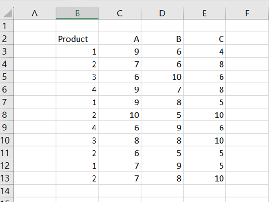
You have a sales report out of four products from one to four and out of three sales regions A, B, and C.
Then you would like to count the standard deviation for the product one in sales region A.
DSTDEV includes three arguments.
Database: the data area B2:E13.
Field: which sales area is investigated A, C2.
Criteria: which product is investigated 1, B2:B3.
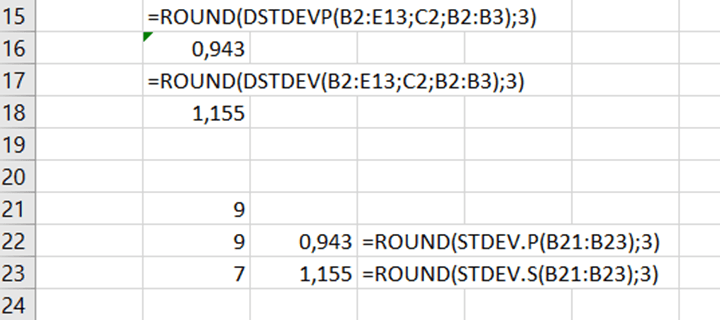
The product 1 has been sold three times in sales region A twice nine pieces and once seven pieces.
The results have been rounded into three decimals.
DSTDEV is for sample and DSTDEVP for population.
How about if you wanted to know the standard deviation for the product 2 in sales region A ? If you select criteria B2:B4, then the function calculates the standard deviation for both products 1 and 2 in sales area A.
In an earlier blog, I have introduced SWITCH function to replace IF. Then a condition was for an exact value, like switch “P1” value to “Jan”.
Now we have bit different SWITCH case. If the value is less than 10, then the returned value is “small”, if the value is from 11 to 14, then returned value is “mid”, the values from 15 to 19 are “fair”, and above, the returned value is “large”.
Earlier, the first argument in SWITCH was cell where the value is, like C4 in our case. However, when we don’t have exact values but less than operator, the first argument is TRUE. Then we have condition if C4 is less than 10, then the returned value is “small”. If C4 is less than 15, then the sentence returns value “mid”. In case C4 value ranges from 15 to 19, then SWITCH returns “fair”. For value 20 and above, the returned value is “large”.
Let’s check a case where we have two input parameters and need to evaluate combination of the two parameters.
Column C may have values 1 or 2, column D may have values a or b. If C equals to 1 and D equals to a, the result is one a. When C is 1 and d is b, the outcome is one b. If C equals to 2 and D a, then result is two a. In case C is 2 and D is b, then the right value is two b.
The key is that for value, we need to combine B4 and C4. Like when combination of B4 and C4 equals to 1a, then the result is one a. Just remember to write value inside parenthesis. Similarly, define all the four combination and the wanted result.
Both IF and SWITCH returned correct values. Still, I prefer SWITCH as we need IF several times and then we need also several parenthesis. When writing a SWITCH sentence, it is easier to have one block in clipboard, paste the block and modify it.
You have a range of cells with values. Then you want to create sum function at the bottom and on the right hand side of the range.
The data range here is B2:E5.
Sum functions are needed in row 6 and column F. This is easy and can be done manually, of course. Just copy the sum to remaining rows and columns.
If you need to do this process repeatedly, a macro might help you. The VBA is added at the end of this blog.
To run the macro, you need to place the cursor in the top left corner of the data range. In our case, the start cell is B2.
Zs is the address of the start cell, eg B2. Then we go at the end of the B row, the address of that cell is stored in zl. Then we go one line down and add the sum sentence SUM(start cell:end cell), then we go one row upwards and one column to right. If that cell is empty then we need to add the sum sentences for each row. If that cell is not empty then we continue counting column sums.
After counting column sums, then we go to the start cell, in this case B2. Zs and zl are populated again. We move to the right end of the data range. Then we move one step to right and there the SUM(start cell:end cell) sentence will be created. Then we move one row down and one column to left. If the cell is empty, then the macro is finished. If the cell is not empty, then we continue counting row sums.
Instead of manually creating sum sentences, place the cursor in B2 and execute the VBA below.
By the way, if you copy the VBA code from website and paste it into Excel VBA editor, and still editor shows syntax errors. When copy pasting the code from application to another, extra spaces might appear in the front of sentence. If something does not work, try to remove tabs or spaces in front of the sentence. Another option is to rewrite the line. Also if you copy the code from website, paste the code first into Notepad. Then copy from Notepad and paste into Excel VBA editor. This might help also.
Before publishing anything, I have tested that VBA works with my Excel.
For good one year, I have followed discussion about LAMBDA function in Excel. Finally the day came, that I found LAMBDA in my own Excel 365. LAMBDA is very versatile function, I just show one example to enjoy the LAMBDA.
If you are working with business-to-business sale persons, they talk prices without value added tax. When I think prices, I think with VAT. So, I need to multiply sales persons’ price with 1,24 to have the prices I understand.
In Excel this can be done in multiple ways.
Write a formula to add 24 % as above.
Another option is to write a custom function. Function is a predefined calculation which returns you a value based on input value(s).
Z_vat is a function. We need to have price to calculate Z_vat. Simply, price multiplied by 1,24 equals to Z_vat meaning the price with value added tax. Save the function in the personal workbook and the custom function is available in all the Excel workbooks.
Use Z_vat as any other function.
Also LAMBDA can be used for calculating value added tax price.
Select formulas and name manager.
The first argument in LAMBDA is price and second price multiplied by 1,24.
This is done with LAMBDA.
In this example, custom function with VBA might have been handier than LAMBDA. Still, LAMBDA offers lots of possibilities. VBA can get long and complex, then LAMBDA is better solution.