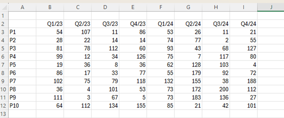
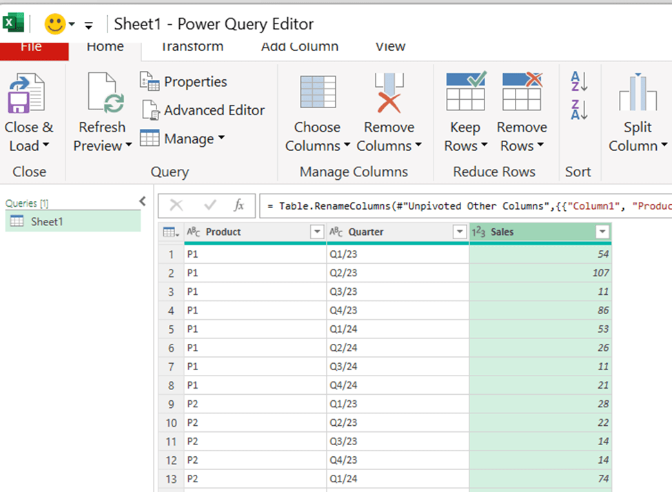
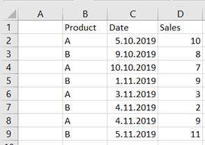
I have extracted data from https://asuntojen.hintatiedot.fi/ about flat prices in Espoo. Can we predict a flat price based on apartment size ?

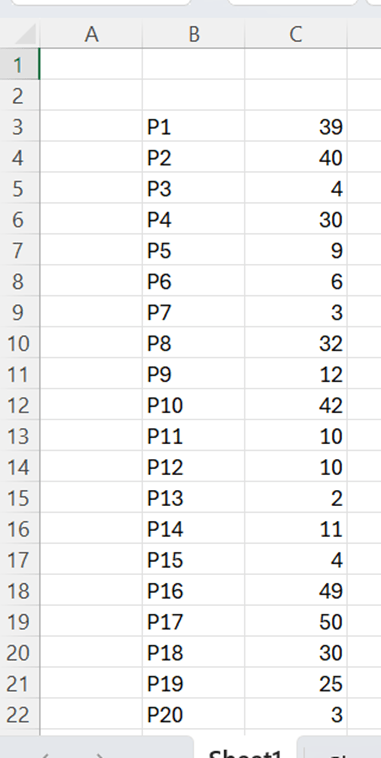
The data consists of 1019 flat prices and apartment sizes. The idea is to check is there  a correlation between flat price based on apartment size. How much should a flat of 400 square meters cost ? The largest flat in the data sample has size of 288 sqm.  How much do the prices vary ?

First, a scatter graph was created. Independent variable, apartment size, was set in X axis and dependent variable flat price in Y axis.

We see visually some trends, the bigger flats get, the wider is also deviation.

The correlation is roughly 0,71. That can be calculated with CORRELATION function. That function includes only two arguments, X values and Y values.

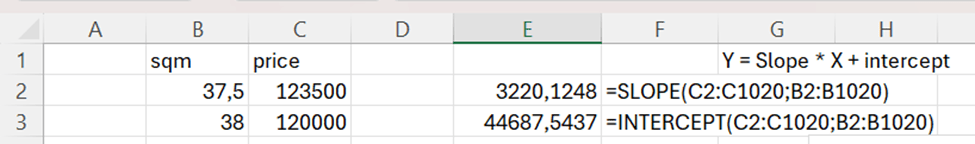
To calculate the trend, we need SLOPE and INTERCEPT functions.

Y = SLOPE * X + INTERCEPT

SLOPE calculates how steep the regression line is and INTERCEPT where Y axis and regression line meet.

Both the formulas have two arguments: values for Y axis and values for X axis.

Another way to have  the SLOPE and INTERCEPT values, is to use LINEST function.

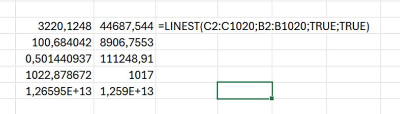
SLOPE and INTERCEPT are in the first row. 0,50 is the R squared value.  The LINEST function returns several values, but SLOPE, INTERCEPT and R squared are useful for us.

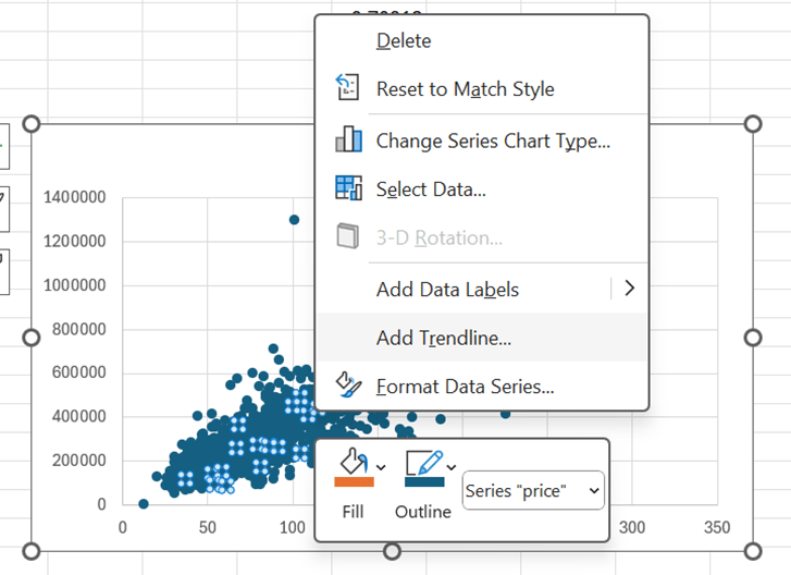
Another way to define the trend line and R squared, it to have right mouse click on top of the scatter graph. The select add trendline.

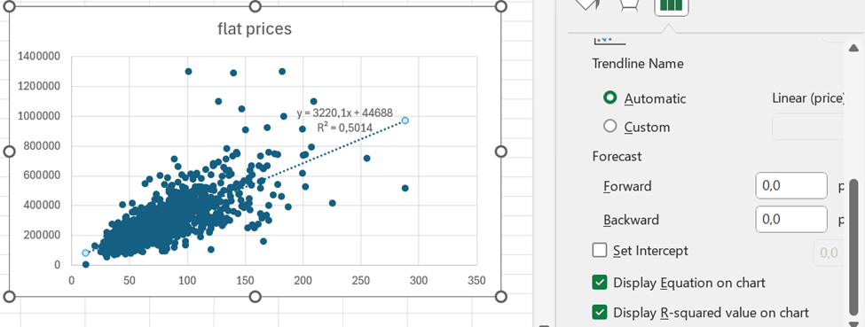
Scroll bit down to see the tick boxes display equation and R squared value. Then the values are visible on the graph.

Based on the equation, the price of the flat with 400 sqm would be appr. 1,3 M€.

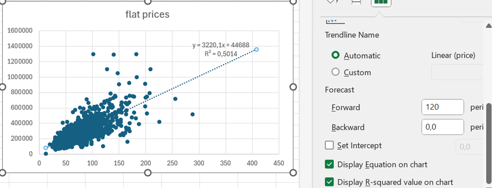
When you format trendline, you can add forward value. 400 sqm flat would cost less than 1,4 M€.

One additional topic is standard deviation. We can see from the graph flats with 50 sqm have less deviation than flats with 147 sqm.

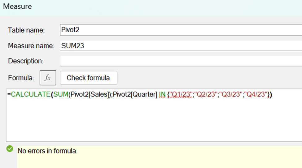
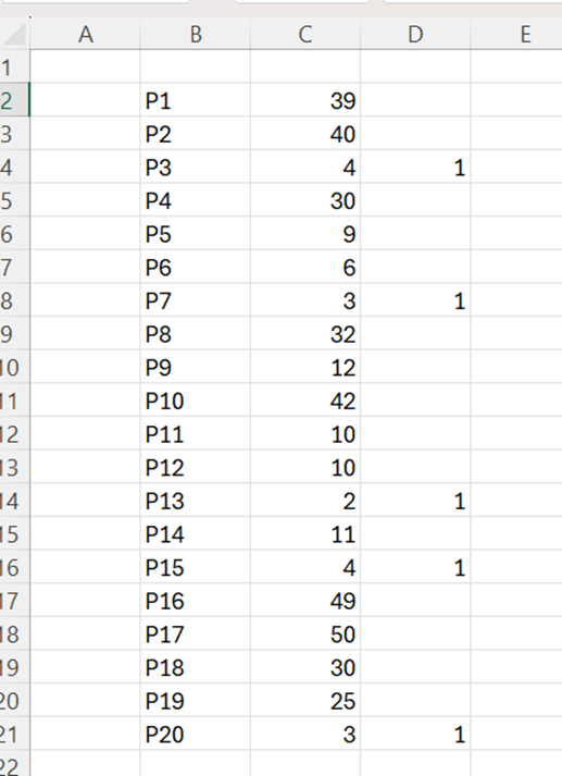
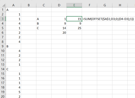
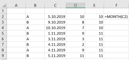
=STDEV.P(IF(ROUND(B2:B1020;0)=E21;C2:C1020))

This is the formula, which counts standard deviation for the flats with specific size. The flat sizes are presented with precision of 0,5 sqm. Therefore, the flat sizes are rounded to full square meter. In E21 cell we have the flat size 50 sqm and in E22 147 sqm.

For a flat with 50 sqm,  the standard deviation is appr. 56,5 k€.

But with flats of 147 sqm, the standard deviation is nearly 280 k€.

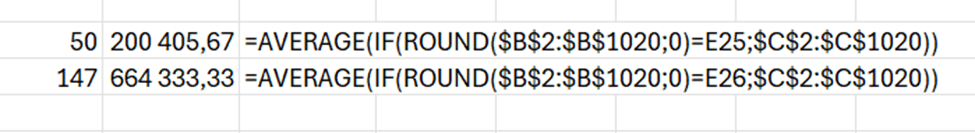
When we count the average price of a flat of 50, that is around 200k€ and for 147 sqm flat around 664 k€. The standard deviations for flats are significant. Therefore, estimate for a flat of 400 sqm, includes variation.

If a flat of 400 sqm costs roughly 1,3 M€, a standard deviation could be around 400 k€.

We have a sales report about products P1 to P10 by quarters from Q1/23 to Q4/24.

Which of the following products saw the largest increase in sales from 2023 to 2024 ?

We can calculate manually the sums for 2023 and 2024 and calculate the change between the years. Sales for P5 have increased mostly when measure the relative change.  

This way we need manual adjustments. We could make a data model and count with DAX.

The data is not in pivot format. The data should include fields product, quarter and sales volume. The data should not be in matrix format.

Download the data into Power Query, activate the first column and then select right mouse button and unpivot other columns.

Now the data is in Pivot format. Add the column headers.

The power query data is loaded into data model. Each row contains product, quarter and sales volume.

Choose close & load to…

Select only create connection and activate add this data to the data model.

Now we have the same data but on top of the data model.

We need the formulas to calculate the year total with DAX.

SUM23 = CALCULATE(SUM(Pivot2[Sales]);Pivot2[Quarter] IN {“Q1/23″;”Q2/23″;”Q3/23″;”Q4/23”})

SUM23 sums the quarters from 2023.

Pivot2 is the table. Sales is the field for sales volumes. Quarter is the time field. Q1/23, Q2/23 and so on are the values in quarter field.

The same pattern works for the total sales in 2024:

SUM24 = CALCULATE(SUM(Pivot2[Sales]);Pivot2[Quarter] IN {“Q1/24″;”Q2/24″;”Q3/24″;”Q4/24”})

Finally, we calculated the change between the years.

Change = ([SUM24]-[SUM23])/[SUM23]

Sales for P5 increased most between 2023 and 2024 compared to other products.

We have the same results but with less manual work. We have the data in data model and DAX was calculating the results. The benefit with data model is, that we can create other measures with DAX on top of the data model.

0000313northp1000010

0000313northp2000300

0000313southp1000010

0000313west0p1000010

0000313east0p3000125

Here I have a sample data extracted form a sales system. The string includes the following data:

1…3     Initial zeroes

4…5     Month, time of sales

6…7     Day, time of sales

8…12   Region, if the region includes four digits, then 12^th digit is zero.

13…14 Product

15…21 Sales quantity with initial zeroes, if needed

This data should be presented in human readable form.

With MID function we can extract certain number of characters from the string. Two functions make the data more readable, PROPER and NUMBERVALUE.

 PROPER makes the first letter capital letter and remaining letters minor letters.

Cell category for B2 and B3 is TEXT. If I refer to B2, like I have done in C2, the cell category for C2 is TEXT. I cannot include those cells in any calculation. When I use NUMBERVALUE function, the result of the function is of cell category number and can be used in calculations.

Back to sample data, I have extracted here the data without PROPER and NUMBERVALUE.

The sentences are:

Month                =MID(B2;4;2) 

Day                     =MID(B2;6;2) 

Region              =IF(MID(B2;12;1)=”0″;MID(B2;8;4);MID(B2;8;5))   

Product            =MID(B2;13;2)             

Amount             =RIGHT(B2;6)

With region, the sentence has to check first whether the 12^th digit is zero, meaning that region is spelled with four digits. Then only four digits are extracted starting from the 8th digit. If 12^th digit is not zero, then five digits are extracted starting from the 8th digit.

The amount could be taken also with MID function, then the sentence would be =MID(B2;15;6).

The result is clear, but the numbers cannot be calculated, and it would look better if regions started with capital letter, and the product were written with capital P.

Now I have used PROPER and NUMBERVALUE functions, and you see the difference immediately.

Texts look better, and even more important, amounts are automatically in calculable format. Also, months and dates are in number category, if you want to calculate, for example, with functions MIN, MAX or AVERAGE.

Month                =NUMBERVALUE(MID(B2;4;2))         

Day                     =NUMBERVALUE((MID(B2;6;2)))      

Region               =PROPER(IF(MID(B2;12;1)=”0″;MID(B2;8;4);MID(B2;8;5)))             

Product            =PROPER(MID(B2;13;2))       

Amount             =NUMBERVALUE(RIGHT(B2;5))        

Typically, PROPER and NUMBERVALUE are nested functions. First you are taking data with functions like MID, and when you have the result, you just frame it with PROPER or NUMBERVALUE. Also, these functions are not only for cosmetic reasons, but also to automatize the calculations.

You have three accounts 30003, 30004 and 30005. The balances are as follows:

               D          C

30003  34          50

30004  34          34

30005  87          21

For 30003 credit is higher than debit. 30004 hold zero balance as both debit and credit are equals. 30005 holds debit balance as debit is higher than credit.

How could we do a report which shows the balances clearly ?

For example, 30003 D is 0 and C 16, 30004 is zero, 30005 D 66 and C 0.

The IF-sentence should be if D is higher than C, then D is D-C and C is zero. If C higher than D, then C is C-D and D is zero.

The sentence in D3 is  =IF(B3>C3;B3-C3;0) and E3 is =IF(C3>B3;C3-B3;0).

Another option to visualize account balances is to define whether balance is debit or credit and what is the balance.

The balance for 30003 is C 16, 30004 is DC 0, and 30005 is D 66.

We avoid some unnecessary zeroes.

The debit or credit is defined with dual IF-sentence. First if is checking if C and D have equal balance, then indication is DC. If this is not the case, but D is higher than C, then the returned value is D, otherwise the value is C.

The sentence in D3 is checking if D equals to C, if so, then the returned value is DC. If D is higher than C, then the value is D, if not, then the value will be C.

E3 is checking if D is higher than C. Luckily, the sentence works also for cases when D is as high as C, returning zero.

Maybe showing summarized balance is more informative than showing both debit and credit balances. All the examples in this blog were done with IF-function.

Values in database are numeric like 1, 23, 587, 3, 56, 78.

When you are writing an SQL query you need to write values between apostrophes and values consist three digits, if the value is with one or two numbers, then initial  zero or two zeroes are needed. Finally values are separated with commas and framed with brackets.

1, 23, 587, 3, 56, 78 are written (‘001′,’023′,’587′,’003′,’056′,’078’). You can do this manually. However, Excel can help you.

If length of the value is one, then at the start we need to add ’00 and after the value ‘. If the length of the value is two, then we need to add ‘0 before the value and ‘ after the value. In case value is three digits long, then only apostrophes are added ‘ before the value and ‘ after the value.

=IF(LEN(C4)=1;”’00″&C4&”‘”;IF(LEN(C4)=2;”‘0″&C4&”‘”;IF(LEN(C4)=3;”‘”&C4&”‘”)))

We do not yet have SQL line.

I added commas after the values apart from the last value. CONCAT formula is creating one string from several cells. CONCAT is merging cells even though the cells would not be in a line.

Only brackets are missing.

Now also brackets are in place.

We can write the query line.  Copy the cell F2 into your SQL editor.

WHERE field1 IN (‘001′,’023′,’587′,’003′,’056′,’078’)

Writing the WHERE line manually is not a big deal, but if you have long list of values, then this blog might be useful. As said earlier, it is nice to have Excel in use, even though it would not be required.  

You have a sales report about twenty products. You need to classify them into four categories based on the sales. A controller may then check the products in the lowest category.

Here we can use QUARTILE formula. Quartile means that we divide the data range into four groups each of them including one fourth of all the values.

So, the controller wants to concentrate on the fourth selling least.

We need to define in the lowest quarter which products have the lowest sales.

To divide data range to quarters happens easily with QUARTILE.EXC function.

The quartile limits are 4,5; 11,5 and 37,25. The function defines just three values as the fourth one is higher than 37,25.

How many product have been selling less than 4,5 ?

We have five product with sales less than 4,5. It would be better if we had a number next to sales representing into which quartile the product belongs. The higher number means higher sales and higher category.

This is the sentence in D4: =IF(C3<=$G$3;1;IF(C3<=$G$4;2;IF(C3<=$G$5;3;4))).

If C3 value is equal or lower than G3, then the value is one. If C3 value is equal or lower than G4, then the value is two. If C3 value is equal or lower than G5, then then the value is 3. In any other cases, the value is 4.

Now the twenty products are divided into four groups, each of them containing five products. The controller may take a closer look at the category one.

Just to double check, we can still count that there are five products in all the categories.

Each of number from one to four appears five times.  Quarterly division works.

Another method to determine the five products with lowest sales, is to use RANK function. Here is a short introduction to RANK.

With RANK we are setting rank order for the values in B3:B7. 8 is the highest with value one, 6 is the second highest with two and so on.

When I add one argument, the rank order is descending, the 8 is the highest with value 5.

The sentence in D2 is =IF(RANK(C2;$C$2:$C$21;1)<=(COUNT($C$2:$C$21)/4);1;””).

If descending rank for the value C2:C21 is lower or equal than number of all the values in C2:C21 divided by four, then value is one. If statement is not true then value is empty.

Excel sets descending rank values for each cell, if the rank is five or less, then value is one, otherwise the value is zero.

This way we can also find five product with lowest sales.

Mode is the value which appears most in data range. For example, in the data range 1, 2, 2, 3 and 4. The mode is two as it exists twice, but all the other numbers exist only once in the data range. Number two has the highest frequency.

Mode is easy to calculate with Excel. Just take the MODE function, the only argument is the data range.

If we have multiple modes in our data range. Both two and four are modes. Still, MODE takes just the first mode. It is true that two is mode but MODE neglects another mode, four.

We have an Excel function MODE.MULT which returns multiple values if there are more than one mode. I wrote the sentence in the cell D2 and pressed enter. Excel automatically populated cells D2 and D3.

MODE.MULT is useful as you never know if there is more than one mode in data range.

One thing to note, as MODE.MULT might populate several cells downwards, it is useful to leave some cells empty below the MODE.MULT.

I was calculating the average in D3 cell. After that, I entered MODE.MULT in D2.

When I pressed enter, this is the result.

Better to do another way round, first average which is taking for sure just one cell. After that enter MODE.MULT.  

The function MODE.SNGL, but that works as MODE.

If you ever need to count which value has the highest frequency in your data range, I recommend you use MODE.MULT. Especially, if you deal with large data sets, and you cannot know whether there are several modes in the data set. Just prepare few cells below the sentence, if MODE.MULT returns several values beneath the sentence.

You have a sales report, and you need to count an average. That’s easy. However, there is one exceptionally high value in the report, 200. That is not a normal value, therefore the average is higher than normal, because of one high sales figure.

One option is to exclude extreme values in the bottom and in the top. The very high sales values will not be counted but also the low values are not considered, either.

Instead of AVERAGE function use TRIMMEAN.

Here is a sales report. As you can see, the last value is considerably higher than other values.

The average for this report is 61.

We would like to exclude the lowest and highest 10 % from the report, then the 200 value would not be counted. Also, the lowest values would also be left out.

The function TRIMMEAN is simple, there are only two arguments data array and percentage.

When we leave the highest 10 % and the lowest 10 % out of average, the trimmed average is 56,1. That is lower than 61, the traditional average. Leaving out the highest and lowest 10 %, is lowering the average because of 200 value.

We can check manually the TRIMMEAN. We need to count 10 % limits manually. Which values TRIMMEAN is excluding from the data range.

The old PERCENTILE function does not exist anymore, now we have PERCENTILE.INC and PERCENTILE.EXC. Both the functions have two arguments: array and percentile. If we want the lowest 10 %, then the percentile is 0,1. For the highest 10 %, the percentile is 0,9.

Now we have percentile limits. If we use PERCENTILE.EXC values, we exclude the values less than 23,3 and higher than 88,5.

Percentile means that below 23,3 are 10 % of observations and above 88,5 are also 10 % of observations. When we count average for sales between the percentiles, that is what TRIMMEAN is doing, I suppose.

Now we need to mark the values in the middle and leave percentile values out. We need an IF sentence which checks that the value is higher than lower percentile limit and lower than high percentile limit. Then the average is calculated only for the values with X.

We take PERCENTILE.EXC values as benchmark, the X should be next to the values which are higher than 23,3 and lower than 88,5.

Now we are counting average for the values with X next to the numeric value. Then we are counting the average for the values when highest and lowest 10 % are excluded. The expected result is same as with TRIMMEAN.

The average for selected values we can do at least in two different ways.

=AVERAGE(IF(C3:C24=”X”;B3:B24))

When using traditional AVERAGE, we need to have nested IF sentence to check where X is set and calculate the average with X marked values.

=AVERAGEIF(C3:C24;”X”;B3:B24)

Excel also has a modern AVERAGEIF function, where IF is embedded and nested IF is not needed. The only arguments area range for criteria, criteria, and average values.

AVERAGEIF is simpler than AVERAGE with nested IF, but both the formulas calculate the same result.

Let’s see do we have the same results with TRIMMEAN and AVERAGE(IF) with PERCENTILE.EXC/INC.

In B6 we have TRIMMEAN for data range 56,1.

In C and D columns we have X if the value is not in highest or lowest percentile. The sentence in C3 =IF(AND(B3>$F$3;B3<$F$4);”X”;””) and in D3 =IF(AND(B3>$G$3;B3<$G$4);”X”;””). In C column X is marked if the value in between F3 and F4. Those values are counted with PERCENTILE.EXC function. In D column we have X if the values are between G3 and G4. In turn, G3 and G4 are calculated with PERCENTILE.INC.

Once the high and low percentiles are marked without X, we can calculate the averages for the values with X. AVERAGEIF and AVERAGE+ nested IF are returning the same values. There is no difference between these two options.

TRIMMEAN returns the value 56,1. The average for PERCENTILE.EXC is roughly 56,06 and for PERCENTILE.INC is 56,25. Differences between averages are minor. PERCENTILE.EXC is closer to TRIMMEAN than PERCENTILE.INC.  No matter which way you calculated the average for selected values, the results are nearly identical. TRIMMEAN is the simplest option.

Have you checked how many different ready made formulas can be found under formulas menu ?

For example, these formulas are under logical section and there is still side bar that some functions are not visible.

I checked duration as I have studied some finance.

Duration means that if you invest in bonds, after how many years you will get back the money you invested in bonds.

You invest 100 € in bonds and you will get 3 % coupon interest annually, means 3 € a year. At the end of maturity 10 years, you will get both invested capital and coupon back 103 €. Market yield is 8 %.

The formula in F2 is =1/(1+$B$6)^D2, meaning 3/(1+1,08)^1. This means the cash flow is discounted with 8 % interest.

G2 has formula =E2*F2. That is the cash flow in present value. H2 has sentence =G2/SUM($G$2:$G$11). H2 calculates percentage of cash flows in present value per year. I2 is =D2*H2. This is year multiplied by percentage of cash flows in present value per year.

Finally, the values in (I2:11) are summed. That value is duration. The investor would get the money invested back in close to 8,5 years. If coupon interest is increased, the duration is decreased, as the investor gets the money back bit faster.

Let’s see how the standard DURATION function under financial functions works.

The arguments for the DURATION function are:

Settlement: start date of the bond.

Maturity: end date of the bond.

Coupon: annual interest rate for the bond.

Yield: discount percentage, the cash flow is discounted to present.

Frequency: how many times a year the coupon interest is paid.

Basis: how many days are in a year. This parameter does not affect much the formula, according to my testings.

The DURATION function returns the same value as value calculated manually. Of course, ready made function is faster and easier. Still, it is useful to understand how function is calculating the values.

DURATION is just one example out of hundreds of formulas in Excel. You might find formulas suitable for your requirements and then you don’t have to enter all the values manually.  

You have an accounting report including account, debet/credit and balance. A part of accounts are with four digits, a part with five. We should calculate total debit and total credit for accounts with five digits.

I tried with SUMIFS without success. Accounts with five digits are including letters, so the numeric condition would not work.

Luckily, SUMPRODUCT did not let us down.

The sentences are here:

=SUMPRODUCT((LEN(B3:B21)=5)*(C3:C21=G3)*D3:D21)

=SUMPRODUCT((LEN(B3:B21)=5)*(C3:C21=G4)*D3:D21)

First, we need to define that we are looking for values with five digits in column B. In column C, we are interested in values in G3 or in G4. After the sentence needs sum-column.  Arguments are separated with multiplication sign.

The same data can be entered in MS Access.

The SQL query is:

SELECT data.dc, Sum(data.balance) AS SumOfbalance

FROM data

WHERE account LIKE ‘?????’

GROUP BY data.dc;

Access return the same results as Excel.

Five digits in MS Access SQL  is ‘?????’, two apostrophes and five question marks inbetween.

Looks like SQL is easier than Excel in this case.

XML is commonly used language. A tag starts with starting tag <TAG> and ends with ending tag </TAG>. The data itself is between the tags.

The example CD catalog was taken from following page XML Examples (w3schools.com) .

The data should be extracted into Excel.

This is the data:

<TITLE>Empire Burlesque</TITLE>

<ARTIST>Bob Dylan</ARTIST>

<COUNTRY>USA</COUNTRY>

<COMPANY>Columbia</COMPANY>

<PRICE>10.90</PRICE>

<YEAR>1985</YEAR>

The data should be extracted like this:

Empire Burlesque

Bob Dylan

USA

Columbia

10.90

1985

Or even better to have name of the segment and data itself in separate columns like this:

TITLE                                            Empire Burlesque

ARTIST                                         Bob Dylan

COUNTRY         USA

COMPANY        Columbia

PRICE                                           10.90

YEAR                                             1985

To extract the data, we can use MID function which extract several characters from the middle of the string.  

MID consists of three arguments:  

1. Text: from which text MID is extracting characters.
2. Start_num: what is the first character to be extracted.
3. Num_char: how many characters are to be extracted.

To extract the segment, can be done with following sentence MID(A3;2;(FIND(“>”;A3))-2.

The extraction is in cell A3,  we are starting from the second character. The number of characters is defined with FIND formula. FIND is looking for the > sign. > is the 7^th character, we need to deduct two from the result. We take five digits starting from second character.

<TITLE>Empire Burlesque</TITLE>

In case the MID returns an error value, we rather have an empty value than an error.

=IF(ISERROR(MID(A3;2;(FIND(“>”;A3))-2));””;(MID(A3;2;(FIND(“>”;A3))-2)))

The sentence to return the data content is more complex.

The first argument, text, is easy. We have the text in A3 cell. The start number is where > is added by one.

<TITLE>Empire Burlesque</TITLE>

In XML above, the data starts with 8^th character.

Number of characters is calculated by finding where / sign. That result is deducted by where > situates. That result is deducted by two. In Empire Burlesque example the / is 25^th character, > is the seventh. 25 minus seven minus two equals 16. The MID needs to extract 16 characters starting with eighth digit as / is the seventh digit and we need to start extracting from the following character.

Just one notification, there are two > signs in the string. FIND function holds the argument start_num, where the find starts. As that is not defined, the FIND returns the value for the first >, which is something we are looking for.

MID(A3;(FIND(“>”;A3)+1);(FIND(“/”;A3)-(FIND(“>”;A3)))-2

In case MID returns an error, the MID can be framed with IF..ISERROR.

=IF(ISERROR(MID(A11;(FIND(“>”;A11)+1);(FIND(“/”;A11)-(FIND(“>”;A11)))-2));””;(MID(A11;(FIND(“>”;A11)+1);(FIND(“/”;A11)-(FIND(“>”;A11)))-2)))

On the top formula text in the cell E3 and below formula text in the cell F3.

You have a sales report and you need to count an average. That’s easy. However, there is one exceptionally high value in the report. That is not a normal value, therefore the average is higher when all the values are counted than without one high sales figure.

One option is to exclude extreme values in the bottom and in the top. The very high sales value will not be counted but also the low values are not considered, either.

Instead of AVERAGE function use TRIMMEAN.

Here is a sales report. As you can see, the last value is considerably higher than other values.

The average for this report is 61.

We would like to exclude lowest and highest 10 % from the report, then the 200 value would not be counted. The old PERCENTILE function does not exist anymore, now we have PERCENTILE.INC and PERCENTILE.EXC. Both the functions have two arguments: array and percentile. If we want the lowest 10 %, then the percentile is 0,1. For the highest 10 %, the percentile is 0,9.

The results with percentile. Exc takes wider values than inc.

Let’s mark manually the values with ‘X’ in the middle when top 10 % and low 10 % are excluded.

The formula in C3 is =IF(AND(B3>$F$3;B3<$F$4);”X”;””). B3 needs to be higher than F3 and lower than F4. Then the value is in the middle and marked with X, not in top 10 % or top low 10 %.

Now, if we calculate the average for the values with X and then TRIMMEAN for the data range, then values should be codirectional.

The average for X marked values are counted in C1 =AVERAGE(IF(C3:C24=”X”;B3:B24)).

Write the sentence and press shift+control+enter not just enter. After pressings shift+control+enter Excel adds arch brackets.

The sentence in D1 is =TRIMMEAN(B3:B24;0,1) . Simply, what is the data range, and what is the percentile. What is proportion of excluded values in data range. In our case it is 0,1, meaning that 10 % should be excluded from top and from bottom.

Both manual average of selected values, marked with X, and TRIMMEAN for data range count pretty similar numbers.

The average of 61 is slightly different than 56, when we excluded exceptionally high and low values. TRIMMEAN is a useful function also in reporting.

If you want to copy something horizontal into vertical or vice versa, you can use paste special and transpose. Excel posses also a function called TRANSPOSE. I demonstrate here a case when to use the function instead of copy – paste transpose.

Activate C2:E2. Place the cursor in B9. Then press control + C. Select home – paste – paste special, activate transpose.

The values inn C2:E2 were copied into B9:B11.

In the same way copy results per region by activating C5:E5. Paste special in C9.

This does not work. The cell C5 calculates the difference between C3 and C4. When the values are copied and transposed in C9, the formula in C9 is A9-B9, which is not our intention.

Now, we can use function TRANSPOSE.

Write the formula =TRANSPOSE(C5:E5) in C9 and press enter. Please note that control + shift + enter is not needed. Just empty values in cells C10:C11.

An advantage with function TRANSPOSE is that values in C9:C11 are dynamic. Let’s change the cost for East region.

The value in C11 changed too.

As the region names in B9:B11 are copied, they are static, not dynamic.

Region name East was changed to West in E2 but the cell B11 is not reflecting.

Also the regions can be populated in B9:B11 with TRANSPOSE function.  Note, that empty first values in B10:B11, that TRANSPOSE is not trying overwrite the values in  B10:B11.

Now both arrays in B9:B11 and C9:C11 are dynamic.

I have introduced INDEX earlier, here is one application how to use INDEX.

Sometimes it nice to calculate manually and check that Excel formula works correctly.

Let’s take matrix calculation with MMULT.

We have two arrays, one in A2:C3 and two in E2:F4.

Write the formula in A7 =MMULT(A2:C3;E2:F4) and press enter.

However, if you want to calculate manually.

The formula in A7 is =A2*E2+B2*E3+C2*E4, in B7 =A2*F2+B2*F3+C2*F4, in A8 =A3*E2+B3*E3+C3*E4 and in B8 =A3*F2+B3*F3+C3*F4.

You can automate the manual process.

Activate the range B2:F4 and rename the range by replacing A2 in the small window. I wrote Mtr as the name for the range.

I have earlier written a blog text about INDEX. You define the range, in this case it is Mrt B2:F4. Coordinates 1;1 refer to B2, coordinates 1;5 to E2.

Formulas in

A6: =INDEX(Mtr;1;1)*INDEX(Mtr;1;5)+INDEX(Mtr;1;2)*INDEX(Mtr;2;5)+INDEX(Mtr;1;3)*INDEX(Mtr;3;5)

B6: =INDEX(Mtr;1;1)*INDEX(Mtr;1;6)+INDEX(Mtr;1;2)*INDEX(Mtr;2;6)+INDEX(Mtr;1;3)*INDEX(Mtr;3;6)

A7: =INDEX(Mtr;2;1)*INDEX(Mtr;1;5)+INDEX(Mtr;2;2)*INDEX(Mtr;2;5)+INDEX(Mtr;2;3)*INDEX(Mtr;3;5)

B7: =INDEX(Mtr;2;1)*INDEX(Mtr;1;6)+INDEX(Mtr;2;2)*INDEX(Mtr;2;6)+INDEX(Mtr;2;3)*INDEX(Mtr;3;6)

An advantage with index with renamed range, the formula strings can be copied as long as range is named after Mtr.

In the picture above the range G2:L4 is named after Mtr.

Recently I have read quite often about XLOOKUP function. Once, after an update, I also got the function in my Excel, I wanted to test the function by myself.

We have a simple sales report. Months are on horizontal axis and product on vertical.

First, we repeat traditional VLOOKUP.

VLOOKUP consists of four arguments.

1. Lookup value: which value to look after, in this case it is P4 in the cell B10.
2. Table array: where to look after the look up value, B3:E6.
3. Column index number: how many steps from B-column you have to take to enter the column where the look up value is, the B column is one. We need to take four steps to check the March values.
4. Range lookup: are we looking after an exact match (false) or a rough match (true). I normally use false just like this time.

If you want that VLOOKUP returns an array, you can add an extra value on top of the return array, like C9 to E9.

If the VLOOKUP does not find an exact match for the lookup value, the formula return #N/A.

This can be tackled with IF and ISERROR functions like:

=IF(ISERROR(VLOOKUP($B10;$B$3:$E$6;E$9;FALSE));”Not found”;(VLOOKUP($B10;$B$3:$E$6;E$9;FALSE)))

Now it is time to introduce our new friend XLOOKUP.

Now it is time to introduce our new friend XLOOKUP.

When you enter the formula, just activate the cell C9.

The arguments for XLOOKUP are:

1. Lookup value: which value to look after, in this case it is P4 in the cell B9. This is similar to the VLOOKUP.
2. Lookup array: list of values containing the lookup value, $B$3:$B$6.
3. Return array: array of the values, in our case sales values, $C$3:$E$6.
4. If not found: if the formula cannot return any value, the formula return this value. “not found.
5. Match code: are we looking after an exact match or a rough match. I use 0 to have an exact match. This is same kind of as range lookup in VLOOKUP.

P5 cannot be found, so the result is “not found”.

When match code is -1, the XLOOKUP returns next smaller value.

Another good thing with XLOOKUP is that it works also vertically, just like HLOOKUP.

Another good thing with XLOOKUP is that as the function returns an array, you can frame with SUM function to get the sum of a row.

XLOOKUP returns an array which is advancement compared to VLOOKUP and HLOOKUP. XLOOKUP makes things easier.

Data is downloaded from web. You should sum up the values you downloaded. However, this does not happen without some modification.

The numeric values don’t get summed.

The cell category is number.

Replacing the space with SUBSTITUTE does not work.

If you replace character number 160, then the thousand separator will disappear. SUM function does not work.

Again the cell category is number, but calculation does not work.

When you frame the previous sentence with VALUE function, the cell gets numeric category and calculation works fine.

=VALUE(SUBSTITUTE(B2;CHAR(160);””))

If you take value from cell with space, the VALUE function does not work.

This is an extension for my earlier OFFSET blog “Introducing OFFSET function”.

One application for OFFSET is selecting a value from a two dimensional report.

On the horizontal axis we have sales areas and products on vertical axis.

The issue is to enter sales area and product, and then receive the correct sales value.

First we need to use MATCH function.

We have list of products in B3:B9. When we want to know what is the ordinal number of the given value. If we enter “F”, is it first, second, third or some other value in the B3:B9 ? The correct value is 5, as the “F” is 5^th letter in the range.

The same applies to the horizontal axis. “West” is the third value in the range C2:E2.

Like this.

Now, we can use OFFSET-function. We know, that F is 5^th and West 3^rd on axises.

In OFFSET-function, we need to first define the starting cell or reference, that is B2. Then we set how many steps we take vertically, that is five steps downwards, as we are looking for “F”. After that we decide step horizontally. We step three steps to right. As we are not expecting a range but a singe cell as the return value, height and width arguments are both 1.

The formula is  =OFFSET(B2;C12;C13;1;1) .

If you want to write the whole formula without interim values the formula goes like this:

=OFFSET(B2;MATCH(B12;B3:B9);MATCH(B13;C2:E2);1;1) .

Replace C12 with MATCH(B12;B3:B9) and

               B13 with MATCH(B13;C2:E2) .

As the OFFSET works with reference plus rows and columns, the examples above are not the only correct ones.

If you set reference as C3, you take one step down and one to right, instead of selecting B2 as the reference.

The OFFSET sentences are:

=OFFSET(C3;C12-1;C13-1;1;1) and

=OFFSET(C3;MATCH(B12;B3:B9)-1;MATCH(B13;C2:E2)-1;1;1) .

I have earlier presented the SUMPRODUCT function.

When PRODUCT is simply same as multiplying cell, SUMPRODUCT is sum of PRODUCTS.

This picture illustrates PRODUCT and SUMPRODUCT functions.

PRODUCT(B3:D3) is same as B3*C3*D3.

PRODUCT(B3:D3)+ PRODUCT(B3:D3) is same as SUMPRODUCT(B3:B4;C3:C4;D3:D4)

A person has a salary of 3000. In the middle of the month the person receives a raise of 240 €.

 In a month there are 22 working days. The persons salary is 3000 during 15 workdays of the month and 3240 for seven working days.

15/22 days the salary is 3000 and 7/22 days 3240. The salary during that month is 3076,36.

That can be calculated with SUMPRODUCT(B4:B5;C4:C5) which might be easier than traditional way in C7.

End of month EOMONTH returns the last day of the month.

However, the function returns the order number since Jan 1^st 1900.

The first argument is date itself, the second is whether the month is before or after the date. 0 means that month to be investigated is the month from the date. In our case the month is January as the date is a January date and the month parameter is zero.

To have more useful value, change the number category to date. You get the format cell box by pressing control + 1.

Now it looks better.

As the month argument is -1, the last date is taken from previous month to given date. Last day of January 2020 was 31^st.

This function looks quite funny, if you just want to know what is the last day of that month.

However, I have found two cases in finance when this function is useful, not only funny.

If you have a high value asset which is depreciated monthly, and you want to calculate depreciation per day. The asset is depreciated more in 31 days than in 30 days.

Asset annual depreciation value is 48 k€, and monthly depreciation is 4 k€. If you want to depreciate per day and depreciation are posted monthly, you need to calculate how many days are in that month.

The first day of the month can be calculated by taking the end of the previous month and adding one day.

Values in cells

D2: =EOMONTH($B$2;C2-1)+1  Last day of the previous month plus one.

E2: =EOMONTH($B$2;C2)  Last day of the month, in this case January.

F2:= =E2-D2+1 Counting the days of the month.

G2: =$B$1/SUM($F$2:$F$13)*F2 Counting the depreciation per day.

The sum F2:F13 is 365 and sum G2:G13 is 48 k sharp.

The same result can be calculated in a bit easier way, too.

The formula in E2 is =DAY(D2), so we just take days from D2. Sentence in F2 is =$B$1/SUM($E$2:$E$13)*E2.

Another possibility for EOMONTH function is statutory reporting, in case you manage your reporting with Excel.

If the reporting day is 3.7.2020, meaning July 3^rd 2020, and you would like to have your reporting period, which is calendar month, automatically populated.

The reporting date is in B3. Supplementary values are in F1:F4.

The start date is defined with supplementary values in B6 and with sentence including embedded values in B7. The same case is with end date in B8 and in B9.

If you want reporting period based on the reporting date, the values are in B11 and B12.

Please note that cells B6:B12 are just values and not numeric fields for further calculations.

B14 and B15 can be used for calculations.

In B15 the sentence ends with +0. This does not change the value, but it changes the result directly to date format.

The sentences are here below for copy pasting.

=”1.”&($F$3)&”.”&($F$4)

=”1.”&(MONTH($B$3))&”.”& (YEAR($B$3))

=($F$2) & “.” & ($F$3) & “.” & ($F$4)

= (DAY(EOMONTH($B$3;0))) & “.” & (MONTH($B$3)) & “.” & (YEAR($B$3))

=”1.” & ($F$3) & “.-” & ($F$2) & “.” & ($F$3) & “.” & ($F$4)

=”1.”&(MONTH($B$3))&”.”& “-” & (DAY(EOMONTH($B$3;0))) & “.” & (MONTH($B$3)) & “.” & (YEAR($B$3))

=EOMONTH(B3;-1)+1

=EOMONTH(B3;0)+0

OFFSET function returns you a range.

Offset-function consists of following arguments:

1. Reference. Where is the starting point of the formula ? In this example it is the cell B2.
2. Rows. How many steps the formula takes downwards from starting point. 1 means, the formula goes to B3.
3. Columns. How many steps the formula takes to the right from B3. One means, the formula ends up in C3.
4. Height: How high is the area starting from C3. Two means the area of C3:C4.
5. Width: How wide is area from C3:C4, three means area C3:E5.

SUM function returns the sum of area C3:E5.

If you want to take steps upwards or to the left, enter negative values.

The same range C3:E5 can be defined in another way too.

To start with D1, you need to go two rows downwards and one column to the left.

=SUM(OFFSET(D1;2;-1;2;3))

OFFSET can be framed with other function than SUM, for example MAX.

When the range is C2:F3, we can check what is the highest value in that range.

=MAX(OFFSET(C2;0;0;2;4))

On the other hand, you can count the same with direct MAX function.

One application how to use OFFSET, is to count values for the sales report which is listing all the sales lines under the header. Range A10:A13 are the sales lines for the material B, valuing 9. The list is dynamic, there might a more a less values under the header.

The first thing is to pick up products which are letters. To pick up alphanumeric fields:

Activate the data area.

Select home – find & select – go to

Press special.

Select Constants radio button and unselect tick boxes apart from Text. Press ok.

Take control + C to copy letters.

Activate wanted destination cell and press control + V.

In order to find where does the area for A or B start, we need MATCH function.

The formula in D3 is =MATCH(C3;$A$1:$A$20). The formula returns the value 1, meaning A is the first cell in range A1:A20. B is 9^th and C 14^th. The last populated cell in column A has order number 20.  The formula in the cell D6 is =COUNTA(A:A).

Now we can calculate the values between A and B.

The formula in D3 is =MATCH(C3;$A$1:$A$20).

From A1 to A20, what is the order number for “A”. That is one, meaning A is in the first cell in the range A1:20.

The formula for D4 is =MATCH(C4;$A$1:$A$20) and for D5 =MATCH(C5;$A$1:$A$20).

D6 shows how many populated cells there are in A-column. The formula is =COUNTA(A:A).

To the point, how to count sales volume for the product A.

The formula in E3 is =SUM(OFFSET($A$1;D3;0;(D4-D3);1)).

The OFFSET starts with the cell A1, that is with absolute reference. We take one step downwards, and no steps to right or left. The are starts in B1 and the area is eight steps of height and one of wide. That area is summed and the result is 15.

The second product B in E4 holds the formula =SUM(OFFSET($A$1;D4;0;(D5-D4);1)). The logic is same as earlier. A1 is the reference cell, then we take 9 steps downwards and zero steps horizontally. The area, to be summed, five steps of height and one step of width. The result is nine.

The same logic applies further also.

In the previous blog, we checked basic loan functions.

If you pay a same payment for your loan every month, then one part of the payment is interest and another part payback of the loan.

To count how much of the payment is interest and how much payback, we will use IPMT and PPMT functions.

If we have a loan of 48 k, interest rate 1,5 % annually, and the payback period is 25 years. Then the monthly payment is around 192 €.

Now we would like to know how 192 € is divided between interest and loan payback.

The A column holds the periods meaning months. The B column includes the interest and C payback amounts. Column D equals to B plus C.

The formula in B4 is =IPMT($C$2/12;A4;$D$2*12;$B$2).

The formula in C4 is =PPMT($C$2/12;A4;$D$2*12;$B$2).

The arguments for the both formulas are:

1. Rate. 1,5 % in C2 must be divided by 12 to get monthly value.
2. Per. Which period is examined. In B4 we check the first period. The reference is relative, when you copy downwards, also the reference changes.
3. Nper. Years needs to be multiplied by 12 to have number of months.
4. Pv. Present value of the loan, amount of the loan is in B2.
5. Fv. Future value, an optional argument.

For example, the first monthly payment of 191,97 € consists of 60 € interest and 131,97 € payback.

To check that the PPMT function works, copy the data down, that you will get all the 300 payments. Then sum up all the PPMTs, you should get 48 k.

As the IPMT and PPMT are to calculate one single period, cumulative interest or loan payback for several periods can be calculated with CUMIPMT and CUMPRINC.

To count how much interest and how much payback you pay during the first year, you can count that with IPMT and PPMT. Just sum B4:B15 and you will get 709,07 € for interest. Sum C4:C15 for payback amount, the result is 1594,57 €.

The same things can be counted with CUMIPMT and CUMPRINC.

The formulas are here for copy pasting:

=CUMIPMT(C2/12;D2*12;B2;1;12;0)

=CUMPRINC(C2/12;D2*12;B2;1;12;0)

The arguments for CUMIPMT and CUMPRINC are:

1. Rate. Interest rate, we divide annual rate by 12 to get monthly rate.
2. Nper. Number of payment periods, 25 years multiplied by 12 to have 300 months.
3. Pv. Present value, amount of the loan taken 48 k.
4. Start_period: From which period we are counting. In this case it is 1.
5. End_period: The last period we are interested in. In this case it is 12.
6. Type: Do the payment take place in the beginning or at the end of the period. We assume at the end.

Functions to calculate loan with Excel can be found in very many Excel sites. I have just collected here the functions I have normally used.

	Function	Argum. 1	Argum.  2	Argum.  3
Calculating the loan amount	PV	Rate	Nper	Pmt
Calculating the interest rate	Rate	Nper	Pmt	Pv
Calculating the pay back period	Nper	Rate	Pmt	Pv
Calculating the monthly payment	Pmt	Rate	Nper	Pv

There are four arguments related to the loan calculation:

1. Monthly payment. (Pmt)
2. Interest. (Rate)
3. Number of periods when loan is paid back. (Nper)
4. Amount of loan. (Pv)

Some functions consist of additional arguments but basic values can be calculated with arguments above.

For the first case, if you want to calculate the loan amount, the function is PMT.

=PMT(Rate; Nper; Pv)

The function in A8 is =PMT(A9/12;A10*12;A11).

The interest rate is defined as annual rate, as we calculate the monthly payment, also the rate should be defined as monthly. Therefore the value in A9 should be divided by 12. Number of periods are years, meaning the loan is planned to be paid back by 25 years. Therefore the periods should be multiplied by 12 to get number of months. Present value is the value of the loan. We are planning to take the loan for 48 k.

To calculate the interest rate for the loan, we will use RATE function.

=RATE(NPER; PMT; PV)

The content in the cell C9 is =RATE(C10*12;-C8;C11)*12.

Number of periods are multiplied to 12 to get the periods by months. The payment in the cell C8 is taken as negative value. The Excel assumes that payments are negative values. As I enter payments as positive values, I will add minus in the formula. The present value, amount of loan, is taken from the cell C11.

Number of periods, meaning how long does it take to pay off the loan, is calculated with NPER function.

=NPER(RATE; PMT; PV)

The cell E10 holds the sentence =NPER(E9/12;-E8;E11)/12.  

First the annual rate is divided by 12. The payment is taken from E8 as negative value because the E8 holds positive value. The loan amount can be found in E11. As the pay back period is understood as years, the whole formula is divided by 12.

The present value, the amount of the loan, is calculated with PV function.

=PV(RATE; NPER; PMT)

The sentence in G11 is =PV(G9/12;G10*12;-G8).

The interest rate is chosen in the cell G9, that is divided 12 to get the monthly interest rate. The number of periods are take in G10 and multiplied by again to get number of months. Finally, payment is extracted in G8 with negative sign.

Please, note that when you calculate with loan functions, the results may vary. Like when you check my screen shot, the present value or loan amount calculated with PV is not exactly 48000 €. When you calculate loan values, the idea with these Excel functions is to give you some idea about monthly payments or interest rate. If you calculate interest rate for your loan by yourself and the check what does you bank say about interest, there might be slight difference.

A sales report is downloaded from ERP.

The dimensions are product, sales date and sales volume.

Sales volumes should be calculated for each product and for each month.

Formulas for copy and paste:

=SUMIFS($D$2:$D$9;$B$2:$B$9;G3;C2:C9;”>=1/11/2019″)

=SUMIFS($D$2:$D$9;$B$2:$B$9;G4;C2:C9;”>=1/11/2019″)

=SUMPRODUCT((B2:B9=G3)*(MONTH(C2:C9)=11)*D2:D9)

=SUMPRODUCT((B2:B9=G4)*(MONTH(C2:C9)=11)*D2:D9)

When using SUMIFS, you need to define first the sum range D2:D9, then product criteria B2:B9, the product is defined in the cell G3. The range for month is C2:C9 the criteria should be “>=1/11/2019”.

SUMPRODUCT is bit more complex, to my opinion. First product dimension is defined in SUMPRODUCT B2:B9 which should equal to G3. Then month in C2:C9 should equal to 11. Finally sum range is marked D2:D9. Multiplication sign is the separator.

Third bit easier option is to create an additional column month to sales report. You can extract month from C2 simply =MONTH(C2) which should return you the value 10.

SUMIFS sentence with additional MONTH column:
=SUMIFS(D2:D9;B2:B9;G3;E2:E9;G9)
=SUMIFS(D2:D9;B2:B9;G4;E2:E9;G10)

If we are looking for number for October, simply stating “>=1/10/2019” in SUMIFS does not work as the statement includes all the values higher or equal to Oct 1^st, including November values. The dates should be limited to higher or equal to Oct 1^st and lower or equal to Oct 31^st.

For SUMPRODUCT changing 11 to 10 is sufficient.

Formulas for copy and paste:

=SUMIFS($D$2:$D$9;$B$2:$B$9;O3;C2:C9;”>=1/10/2019″;C2:C9;”<=31/10/2019″)

=SUMIFS($D$2:$D$9;$B$2:$B$9;O4;C2:C9;”>=1/10/2019″;C2:C9;”<=31/10/2019″)

=SUMPRODUCT((B2:B9=O3)*(MONTH(C2:C9)=10)*D2:D9)

=SUMPRODUCT((B2:B9=O4)*(MONTH(C2:C9)=10)*D2:D9)

=SUMIFS(D2:D9;B2:B9;O3;E2:E9;O9)

=SUMIFS(D2:D9;B2:B9;O4;E2:E9;O10)

This is not really a part of the header, but the same things what was done with SUMIF and SUMIFS can be tackled with Pivot tables too.

First, we need header row.

Activate the data area B1:D9 and select insert – pivot table.

INDIRECT formula returns the value of a defined cell. Examples below shed the light how the function functions.

Think you have a three-dimensional sales report Excel sheet. In each sheet there is a sales report from different sales district. The top sheet sums up all the sheets.

The top sheet sums up districts 1 to 10.

But somewhere exists an error and the top sheet cannot calculate the sum.

You can browse each sheet and track the error. If you do this several times or if you have dozens of sheets in your workbook, you might think to have a faster way to find out the sheet not functioning correctly.

INDIRECT formula will help us. We need to what is the cell C7 value in each sheet, as one C7 shows an error.

In the District_1 view the value in C7 is 47,2 in District_2 C7 holds value of 27,6 and so on. The faulty value is in sheet District_7.

Once the wrong value was corrected, the sheet District_7 shows correct figures.

The INDIRECT formula needs sheet, exclamation mark and cell like INDIRECT(District_1!C7). With references you avoid typing the formula each time.

=INDIRECT($B16 & “!” & C$15 & “”)

To have extra spaces in Excel cell is quite common issue. Especially when data is downloaded from another system to Excel, some additional digits can be found in Excel.

I have had issues with leading spaces. Here are some hints how I have tackled the space issues.

First thing is to check how many digits the cell contains as the initial spaces are not visible. The function LEN is for this purpose.

The formulas, which are worth trying first, are TRIM and CLEAN. SUBSTITUTE is to change a specific character to another. If you want to use REPLACE, you need to know which digit, like the first one, is space.

One option to delete leading space or two leading spaces, is to write IF sentence. If the first two digits are spaces, then take digits from the 3^rd onward. Number of digits to be captured is the total length of the cell minus two. If cell contains only one leading space, then Excel should capture digits starting from the second one, and count the last digit by taking the total length minus one. If neither of IF statements, the first two digits are spaces or the first digit is space, is true, then IF is returning the cell value unmodified.

=IF(LEFT(C18;2)=”  “;MID(C18;3;(LEN(C18)-2));IF(LEFT(C18;1)=” “;MID(C18;2;(LEN(C18)-1));C18))

The issue with space is that space is not in fact a space. Each digit is Excel has a CHAR number. Like capital A is char(65). Function CODE returns the char number.

In Excel there is char(160), which is like space but not exactly space. Space + abc is not similar to char(160) + abc. Similar formulas with work with the first case might not work with the second one.

The best solution so far I have found with extra spaces have been nested function to link several function and hopefully some of the works. When you create a customized formula, you don’t have to write whole chain every time from the start till end.

Function z_space2(z_cell)

z_space2 = WorksheetFunction.Trim(WorksheetFunction.Clean(WorksheetFunction.Substitute(z_cell, Chr(160), ” “)))

End Function

We have a two dimensional table with unique axis.

This example is simplified from real case. The user wants to know the value by entering values from both the axis. Like pr1 and south should return the value 2.

We need two formulas for this case, MATCH and INDEX. Both the formulas are relatively simple.

In the list f is the fourth letter.

INDEX forms coordinates for the range.

Range(B3:D5) forms an array. B3 is a corner where you start counting row and columns. First row and third column is D3 and value 6. Second row and first column is B4, the value 2.

Entering values are in fields G2 and G3. The pr3 is searched in B4:B6 with MARCH, and west in C3:E3, also with MATCH. Then INDEX is using the values form MATCH functions to find out the value for pr3/west which equals to 9.

Both INDEX and MATCH are embedded in G8.