You have a sales report. We need to make a distribution graph, a histogram, like how many values are equal or less than five, how many values are higher than five but less or equal to ten and so forth.
Our sample data is very simple, that we could see the correct results immediately.
The sentence in E3 is =COUNTIFS($B$2:$B$11;”>”&D2;$B$2:$B$11;”<=”&D3) .
The COUNTIFS is used here with two criterias. The formula is counting how many values in the data range are higher than D2 and lower or equal to D3. Bit tricky part is define the cell reference “>”&D2.
Another option is to use FREQUENCY function.
Enter the data array B2:B11 and bin arrays D3:D6. Then write the formula in E3 and hit enter.
You will get the frequencies per bin.
The third option is to use analysis toolpak. You need to download analysis toolpak via Excel options.
Press go.
Choose analysis toolpak and press ok.
After that, I have a data analysis button far right under data view.
Write again data array and bin arrays.
Press data analysis under data view.
Select histogram and press ok.
Enter input range, bin range and output options. Activate also the chart output. Press ok.
The result.
The COUNTIFS is more complex than FREQUENCY or data analysis. Data analysis is practical once it is loaded. Excel is offering various ways to calculate and present histogram.
You have a time series graph with first actual figures and then planned figures. The actual and plan needs to be graphically separated, that the audience would immediately see which figures are actuals and which are planned ones.
In the graph there is just one line, first part represents the actual figures and the end of he line, planned figures.
Actual figures and planned figures are in different columns, therefore they can have different headers.
I have value in D18, that is the last actual number, but the graph looks better when we have both values in last actual row.
Activate the range B2:C21 and take insert – charts.
Select one chart template.
Actual figures are in graph.
Select B2:B21;D2:D21, take copy like control + C.
Click right mouse button on top of the graph and select paste special.
These selections are ok.
The result.
Maybe a bright red would be a more striking colour for the planned figures.
Click the planned figures and take color under format data series.
If you want to change chart type from the line, take right mouse button and change chart type.
Select combo from left side. Chart type can be defined per series. If you want to have actuals bars and planned figures as line.
It is possible to have two different chart types like bar and line. However, I prefer the same chart type for actual and planned figures.
Click the chart and press plus button, then select chart title. You can edit the title.
Now we have header for the graph.
The legeds blue actual and red planned would clarify the graph.
Click the graph and press plus in the top right hand corner.
Select legend.
Now the graph looks like what I was planning to have. Actual values are in blue line and planned values are in red line. Legend is clarifying which one is which.
Excel is a tool for presenting not only calculations.
You have a sales report, and you need to count an average. That’s easy. However, there is one exceptionally high value in the report, 200. That is not a normal value, therefore the average is higher than normal, because of one high sales figure.
One option is to exclude extreme values in the bottom and in the top. The very high sales values will not be counted but also the low values are not considered, either.
Instead of AVERAGE function use TRIMMEAN.
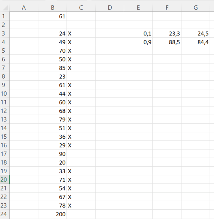
Here is a sales report. As you can see, the last value is considerably higher than other values.
The average for this report is 61.
We would like to exclude the lowest and highest 10 % from the report, then the 200 value would not be counted. Also, the lowest values would also be left out.
The function TRIMMEAN is simple, there are only two arguments data array and percentage.
When we leave the highest 10 % and the lowest 10 % out of average, the trimmed average is 56,1. That is lower than 61, the traditional average. Leaving out the highest and lowest 10 %, is lowering the average because of 200 value.
We can check manually the TRIMMEAN. We need to count 10 % limits manually. Which values TRIMMEAN is excluding from the data range.
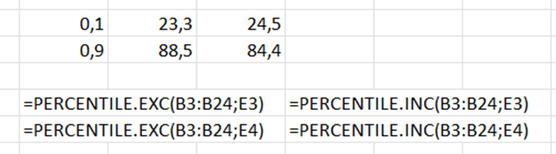
The old PERCENTILE function does not exist anymore, now we have PERCENTILE.INC and PERCENTILE.EXC. Both the functions have two arguments: array and percentile. If we want the lowest 10 %, then the percentile is 0,1. For the highest 10 %, the percentile is 0,9.
Now we have percentile limits. If we use PERCENTILE.EXC values, we exclude the values less than 23,3 and higher than 88,5.
Percentile means that below 23,3 are 10 % of observations and above 88,5 are also 10 % of observations. When we count average for sales between the percentiles, that is what TRIMMEAN is doing, I suppose.
Now we need to mark the values in the middle and leave percentile values out. We need an IF sentence which checks that the value is higher than lower percentile limit and lower than high percentile limit. Then the average is calculated only for the values with X.
We take PERCENTILE.EXC values as benchmark, the X should be next to the values which are higher than 23,3 and lower than 88,5.
Now we are counting average for the values with X next to the numeric value. Then we are counting the average for the values when highest and lowest 10 % are excluded. The expected result is same as with TRIMMEAN.
The average for selected values we can do at least in two different ways.
=AVERAGE(IF(C3:C24=”X”;B3:B24))
When using traditional AVERAGE, we need to have nested IF sentence to check where X is set and calculate the average with X marked values.
=AVERAGEIF(C3:C24;”X”;B3:B24)
Excel also has a modern AVERAGEIF function, where IF is embedded and nested IF is not needed. The only arguments area range for criteria, criteria, and average values.
AVERAGEIF is simpler than AVERAGE with nested IF, but both the formulas calculate the same result.
Let’s see do we have the same results with TRIMMEAN and AVERAGE(IF) with PERCENTILE.EXC/INC.
In B6 we have TRIMMEAN for data range 56,1.
In C and D columns we have X if the value is not in highest or lowest percentile. The sentence in C3 =IF(AND(B3>$F$3;B3<$F$4);”X”;””) and in D3 =IF(AND(B3>$G$3;B3<$G$4);”X”;””). In C column X is marked if the value in between F3 and F4. Those values are counted with PERCENTILE.EXC function. In D column we have X if the values are between G3 and G4. In turn, G3 and G4 are calculated with PERCENTILE.INC.
Once the high and low percentiles are marked without X, we can calculate the averages for the values with X. AVERAGEIF and AVERAGE+ nested IF are returning the same values. There is no difference between these two options.
TRIMMEAN returns the value 56,1. The average for PERCENTILE.EXC is roughly 56,06 and for PERCENTILE.INC is 56,25. Differences between averages are minor. PERCENTILE.EXC is closer to TRIMMEAN than PERCENTILE.INC. No matter which way you calculated the average for selected values, the results are nearly identical. TRIMMEAN is the simplest option.
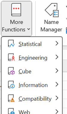
Have you checked how many different ready made formulas can be found under formulas menu ?
For example, these formulas are under logical section and there is still side bar that some functions are not visible.
I checked duration as I have studied some finance.
Duration means that if you invest in bonds, after how many years you will get back the money you invested in bonds.
You invest 100 € in bonds and you will get 3 % coupon interest annually, means 3 € a year. At the end of maturity 10 years, you will get both invested capital and coupon back 103 €. Market yield is 8 %.
The formula in F2 is =1/(1+$B$6)^D2, meaning 3/(1+1,08)^1. This means the cash flow is discounted with 8 % interest.
G2 has formula =E2*F2. That is the cash flow in present value. H2 has sentence =G2/SUM($G$2:$G$11). H2 calculates percentage of cash flows in present value per year. I2 is =D2*H2. This is year multiplied by percentage of cash flows in present value per year.
Finally, the values in (I2:11) are summed. That value is duration. The investor would get the money invested back in close to 8,5 years. If coupon interest is increased, the duration is decreased, as the investor gets the money back bit faster.
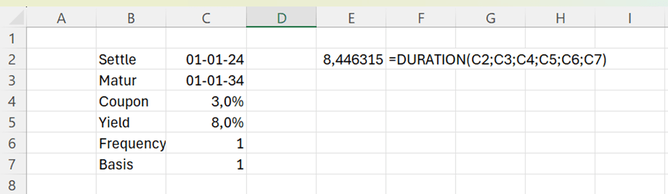
Let’s see how the standard DURATION function under financial functions works.
The arguments for the DURATION function are:
Settlement: start date of the bond.
Maturity: end date of the bond.
Coupon: annual interest rate for the bond.
Yield: discount percentage, the cash flow is discounted to present.
Frequency: how many times a year the coupon interest is paid.
Basis: how many days are in a year. This parameter does not affect much the formula, according to my testings.
The DURATION function returns the same value as value calculated manually. Of course, ready made function is faster and easier. Still, it is useful to understand how function is calculating the values.
DURATION is just one example out of hundreds of formulas in Excel. You might find formulas suitable for your requirements and then you don’t have to enter all the values manually.
Standard deviation 1 = standard deviation of security 1
Portion 2 = percentage of security 2 in portfolio
Standard deviation 2 = standard deviation of security 2
Correlation = Correlation between security 1 and security 2
We have two securities in our portfolio, A and B. Expected return for A is 5 % and standard deviation is 8 %. Expected return for B is 15 % and standard deviation is 18 %. Security A is clearly a low-risk investment compared to security B. The mutual correlation is 12 %.
You can calculate standard deviation just like this:
=(C3^2*C5^2+2*C3*C5*D3*D5*C6+D3^2*D5^2)^0,5
If you calculate this repeatedly, it is useful to create your own function.
We are calculating the value for z_port. For that we need five input values p1, s1, p2, s2 and co.
Input arguments are:
P1 = percentage of security 1 in portfolio
S1 = standard deviation of security 1 i
P2 = percentage of security 2 in portfolio
S2 = standard deviation of security 2
Co = Correlation between security 1 and security 2
You need to enter five input arguments to calculate the standard deviation.
Let’s calculate also the expected return.
It is simple
P 1 = percentage of security 1 in portfolio
R 1 = expected return of security 1 i
P 2 = percentage of security 2 in portfolio
S 2 = expected return of security 2
The custom function would be:
Function z_ret(p1, r1, p2, r2)
z_ret = p1 * r1 + p2 * r2
End Function
Writing a custom function for expected return does not save so much time compared to calculating the same manually. Still, it is a neat presentation to have a custom function.
Both manual counting and custom functions return the same values.
We are investing in a two-security portfolio. Our investment policy is to be risk averse, meaning that we prefer to have a portfolio with as low risk as possible. We need to minimize the standard deviation. Intuitively, we should invest all the money in security A and nothing in security B.
In our case also the correlation plays a part as correlation is low, it means that we can effectively diversify risk by investing in both the securities.
When correlation is low, it is possible that when value of one security is decreasing, the value of another might be increasing. The total value of the portfolio would not decrease that much.
We have a matrix with proportions of A and B securities with an interval of 10 %. Then we have standard deviation and expected return with those proportions. We can see in the matrix that standard deviation is dropping a bit when we increase the proportion of security B in our portfolio.
The sentence in D11 is =z_port(B11;$C$5;C11;$D$5;$C$6) and in E11 =z_ret(B11;$C$4;C11;$D$4).
We draw a graph by selecting the data range. Just untick B in the left box as we want B to be horizontal axis. Press “edit” in the right box and select value 0%-100% under B.
We see in the graph that standard deviation is dropping slightly as we increase the proportion of security B in our two-security portfolio. Expected return is linear.
When we include more of security B in our portfolio, the expected return increases. The optimized portfolio is not only of lower risk but also the expected return is higher than investing everything in security A.
If you don’t have yet solver add-in in Excel, you can activate that in Excel options.
Then solver appeared under data ribbon. In my Excel it is in the furthest right corner.
We want to minimize the portfolio standard deviation I4 by changing the proportion of security B E4.
Solver found results.
If we invest 13 % in security B and 87 % in security A, we have the lowest risk level, minimum variance portfolio. Also, the expected return is more than 6 %, that is more than what we would expect by investing in security A only.
Now A and B are not correlating with each other much. Let’s change the calculation and increase the correlation to 60 %.
Solver is proposing to invest only in security A. There would not be diversification between A and B, but everything would be invested in A. Then the expected return is 5 %.
Let’s drop correction to negative -5 %.
18 % should be invested in security B, also expected return is higher than in earlier scenarios.
When correlation is slightly negative, the portfolio turns out to be more profitable with less risk.
The graph is drawn with the assumption that correction is – 5%. We can see from the graph that our portfolio is having lower standard deviation but higher profit.
If you invest in two different securities, it is better to choose the couple that correlates as less as possible with each other.
Another takeaway is the solver. If you need to find an optimal solution for some calculations, test the solver. We wanted to find the minimum value of one parameter by changing the other parameter.
After playing cards, you will count points of all the cards you have at hand. Ace is 14, king 13, queen 12 and jack 11. Number cards have the value according to number. The one who has the highest or lowest score is the winner.
It is easy to count but only picture cards have letters, which need to be converted to numbers.
Excel can help you or at least make counting a bit faster.
First we are introducing the variables. Z_val is the value of cards. Z_start is the address of the starting cell address. Z_val is set to zero. The program starts going downwards the cells. If the cell contains A then 14 is added to z_val, K is 13, Q is 12 and J is 11.
The number cards have their own value, like 6 is 6 and 7 is 7. To define which cell contains the numeric value, we can use Excel function ISNUMBER. In Visual Basic we can use Excel functions with WorksheetFunction extension.
The macro goes downwards cell by cell adding the sum value z_val, till the macro hits the first empty cell. Then macro jumps back to start cell and enter the sum value z_val into cell one above the start cell z_start.
Here is the macro:
Sub z_cards2()
Dim z_val
Dim z_start
z_val = 0
z_start = ActiveCell.Address
Do Until ActiveCell.Value = “”
If ActiveCell.Value = “A” Then
z_val = (z_val + 14)
ElseIf ActiveCell.Value = “K” Then
z_val = (z_val + 13)
ElseIf ActiveCell.Value = “Q” Then
z_val = (z_val + 12)
ElseIf ActiveCell.Value = “J” Then
z_val = (z_val + 11)
ElseIf WorksheetFunction.IsNumber(ActiveCell.Value) Then
z_val = (z_val + ActiveCell.Value)
Else
z_val = z_val + 0
End If
ActiveCell.Offset(1, 0).Select
Loop
Range(z_start).Select
ActiveCell.Offset(-1, 0).Select
ActiveCell.Value = z_val
End Sub
In B6 we have a value which does not have any value in our calculations as there is no Z-card in playing cards.
Place the cursor in B4 and execute the macro.
Z-card was not counted. If you mistakenly enter a wrong letter, the macro can handle that by passing the cell.
Excel macro was counting the points for each player. Of course, you could have done that manually too, but Excel can be used also for counting playing card points.
If value is equal to average value, then the result is ave, if value is not average and if the value is above average then the result is above, if the value is not in average and it is below the average, then the result is below.
The conditional formatting has also feature above and below average. If you select the data range C3:C12 and select home – conditional formatting – top/bottom rules – above average, then the values higher than average are highlighted.
The cells above the average are coloured. The same cells are highlighted as with IF sentence.
You can count the values above average with MS Access.
Table Ave was created.
The table consists of sales rep and sales amount. ID field is a running number.
Same data is entered as in Excel was keyed in Access.
An SQL query is written to detect the values below and above average. The logic is same than in Excel. In Access if is IIF.
SELECT sales,
IIF(sales = (SELECT AVG(sales) FROM ave), ‘avg’, IIF(sales > (SELECT AVG(sales) FROM ave), ‘above’, ‘below’))
FROM ave;
The results are the same as in Excel.
When comparing these three methods, I think that conditional formatting is the easiest and fastest way to calculate which values are above or below average. No manual logic is needed when conditional formatting is used. Normally, Access is not used for calculation like this, but SQL is a very powerful tool for many analytical tasks.
I have blogged how to count values in the data range, like how many times letter “A” appears in the data range. Let’s take such a large data range that it does not fit Excel workbook.
I have a text file with good 3M rows of values. Each line holds value either A, B, C, or D.
How many times does the letter “A” exists in the file ? We cannot count with normal Excel COUNT. As the data does not fit normal Excel workbook.
3M rows were loaded into Excel data model.
We use COUNTA function in DAX.
The formula is: =COUNTA(C3M[Val]) .
C3M is the table and Val field.
Pivot settings.
The results per letter.
Next step is to count percentual division between four letters. Therefore, we need to count the total number of rows.
The formula is: =calculate(COUNT(C3M[Val]),ALL(C3M))
The CALCULATE formula calculates the total number of rows in the data range.
To have the percentage distribution, we need to just divide count of each letter by total number of rows. To have the percentage value, the format is percentage.
The formula is: =divide([Count],[Count_all]) .
We divide one measure with another.
The letter A counts for a half, other letter divide the remaining half.
Count_all measure is counting with CALCULATE the total number of records. The expression for CALCULATE is table C3M and field Val, the filter is ALL as we are counting all the records in the table.
One option is again to use MS Access, as Access can take 3M rows of data.
The table has two fields running number and the letters in VAL field.
A simple SQL query, just remember the square brackets around the table.
The results in absolute number.
Here is the SQL query to count percentage values. How many percents of all the letters is letter “A” ?
SELECT C3M.Val, ROUND(Count(Val)/(SELECT COUNT(*) FROM [C3M]), 2) AS Expr1
FROM C3M
GROUP BY C3M.Val;
Now the square brackets were not needed with FROM command. To have percent values, we need to take the total number of letter “A” rows with Count(Val). That is divided with all the records in the table (SELECT COUNT(*) FROM [C3M]). In order to decrease the number of decimals, ROUND function is framing the division calculation.
Every second letter in the data range is “A”. Remaining letters B, C, D are dividing evenly remaining half.
SQL is powerful tool to calculate numeric values out of a large data. When using DAX we needed few formulas, but with SQL we needed only few lines. In case you want to present distribution of the four letters, you can easily create a graph like this in Excel.
You have a sales report. Each sales rep from A to J have sold a number of products except D and H.
We should count the average sales.
The standard average formula counts only numbers. For example, sales reps D and H are not included. Sum of numbers is 447. If you divide that with eight, that is roughly 56.
When sales reps D and H are on the payroll, they need to be included in the average counting. 56 is too high average as two sales reps have zero sales.
Data includes NULL values.
The more realistic average is around 45.
To make denominator as ten, we have few options available.
We can count cell with value in B1:B10 and then add cells without value B1:B10 to include all the cells. Also ROWS function counts rows in data range.
We count the sum in B1:B10 and then we divide by COUNT + COUNTBLANK or by ROWS -function. Then we have the wanted 45 as a result.
Another option is to populate NULL values with zero numbers, then standard average can be used.
Activate the B1:B10 range and execute the macro below.
Sub z_zero()
Dim cell As Range
For Each cell In Selection
If cell.Value = vbNullString Then
cell.Value = 0
End If
Next cell
End Sub
NULL values are in Excel VBA called as vbNullString. If the macro finds NULL value in the range, then that is replaced by zero. If the value is zero, then it is NULL.
Activate the values, then execute the macro. Now NULL values have been replaced by zero, and standard AVERAGE behaves as we want.
We can count average in Access too.
The same values are in Access.
A query was created.
The SQL is:
SELECT Avg(IIf(IsNull(sal),0,sal)) AS Expr1
FROM tab;
The result is the same as in Excel.
We have nested formulas AVG, IIF and ISNULL. In other SQL dialects same thing can be done with AVG and IFNULL.
SQL sentence is short compared to do same in Excel. Excel is a better tool number crunching, but if you can do something with SQL, Access is worth trying out.
You have in Excel cells with different colours. Now the colours are not cosmetics but colours play part when we are counting sums and counts.
First, we need to count how many cells are coloured with certain colours. Like how many cells are having yellow colour ? That is still easy to count visually.
How many different colour can you see ? The issue is that there are several shades of green. What is the frequency of each colour ?
The solution is interior.colorindex property. That is a number which is unique for each colour. We need to have a macro which is checking the colorindex and printing the number to the next cell. Then we can count how many times each number is appearing in the data range.
In Visual Basic editor we have the immediate window. There we can query cells properties like interior.colorindex. We have the cursor in a yellow cell. The colorindex for yellow colour is six.
A macro may check each cell and print the colorindex value.
Sub z_colors()
Dim zc
Do Until ActiveCell.Interior.colorindex = -4142
zc = ActiveCell.Interior.colorindex
ActiveCell.Offset(0, 1).Select
ActiveCell.Value = zc
ActiveCell.Offset(1, -1).Select
Loop
End Sub
Macro to define colorindex for each cell is relatively simple. The cell without any interior colour has colorindex -4142. The macro is going downwards and storing the colorindex as zc variable. Then macro takes one step right and pastes the number at the right hand side of the cell. The macro takes the next cell in the range. When macro finds the cell with interior colorinxed -4142, then the macro stops there.
The cursor was placed in B3 and the macro was executed. As you see, most of the green cells have 43 as colorindex but one has 50.
Note also that the numbers are not dynamic. If you change the interior colour, you need to execute the macro again.
Copy paste the number and take data – data tools – remove duplicates.
Press ok.
Four unique values remain.
With COUNTIF we can calculate how many times each number exits in the number range.
Still, it might be difficult to map colorindex number and colour.
Sub z_colors2()
Dim zi
Do Until ActiveCell.Value = “”
zi = ActiveCell.Value
ActiveCell.Offset(0, -1).Select
ActiveCell.Interior.colorindex = zi
ActiveCell.Offset(1, 1).Select
Loop
End Sub
This macro fills the cell left from the colorindex number with colour related to colorindex.
Place the cursor in the cell G3 and execute the macro. The macro will colour the cells in the column F.
The data range includes ten cells with yellow interior, two reds, five greens and one turquoise.
How about if coloured cells include values.
We need to count sum based on the interior colours, like what is the sum of the values in red cells.
We can use the same colorindex number, but now we use SUMIF function.
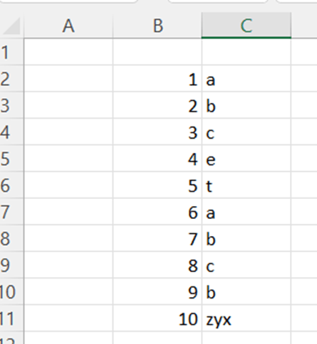
In my earlier blog I showed how you can count how many times a certain character exists within a data range. Regrettably, I forgot to present how you do that in Microsoft Access. All my examples were in Excel.
Same data, as in earlier count find blog, is entered in Access. ID is just a running number with AutoNumber data type. Column Val consists of the values we are interested in.
How many times eg. letter A exists in the data range ?
In query part, we create following query:
SELECT Val, COUNT(Val)
FROM [Table]
GROUP BY Val
ORDER BY COUNT(Val) DESC;
We select values in Val column and the counted number of Val column values. Note that table needs to be in square brackets. We are grouping by the Val field. Finally, results are in descending order by counting val-column results.
The results are the same as in Excel. Letter A exists five times in the data range.
If you don’t have square brackets around the table, you will get a syntax error message.
If you don’t want to see all the results but only the highest two values, you can add TOP command in the start of SELECT query.
Limiting the results to the first values exists in other SQL tools but is different. It can be like WHERE rownum < 3 or LIMIT 2.
Result:
The result is same as earlier but now only two first values are listed.
Counting how many times a letter exists in a data range, can be done quickly in Access. If you get the data into Access first, then creating a query is simple.
You have scatter diagram, where you have nine dots. Each dot has value on X and Y-axis.
To draw a graph, activate the data range B2:C11, select under insert menu a scatter graph.
Now you have graph with dots.
It would be easier to identify each dot with a letter.
Write the dot identifiers in A column.
Activate the dots in the graph and click right mouse button. Then select add data labels.
Press select range and activate name range from A3 onwards.
If you inserted an extra dot in graph, which ones of the existing dots would be the closest to the extra dot ?
The value is defined by counting obs x value minus dot’s x value. That value is squared. Then obs y value and dot’s y value. That also is squared. Then we sum two values and take root square. This is repeated for all the dots.
The sentence in D3 is =SQRT(($B$12-B3)^2+($C$12-C3)^2). That is copied down till D11.
When we have values, we should rank the number. Let’s take top three dots. This we can do with RANK.EQ function.
Here is a simple example about RANK.EQ formula. Just enter the value and range. The highest number has first rank.
If we want to take just three biggest numbers, we add an IF sentence.
The formula in C3 is =IF(RANK.EQ(B3;$B$3:$B$7)>3;””;(RANK.EQ(B3;$B$3:$B$7))). Note that this is counting highest as the first value.
If the lowest number is the first, then you need to add one more argument with value one.
Then we need IF-sentence to take three lowest numbers.
The sentence in C3 is =IF(RANK.EQ(B3;$B$3:$B$7;1)>3;””;(RANK.EQ(B3;$B$3:$B$7;1))).
When we implement this logic to our original Excel, it looks like this:
The sentence in E3 is =IF(RANK.EQ(D3;$D$3:$D$12;1)>3;””;RANK.EQ(D3;$D$3:$D$12;1)).
That is copied down to E12.
As you can see from the graph, the closest points for the OBS are G, H and F.
One application of this functionality is if we want to define attributes for OBS, then attributes of G, H and F are also the closest attributes to OBS.
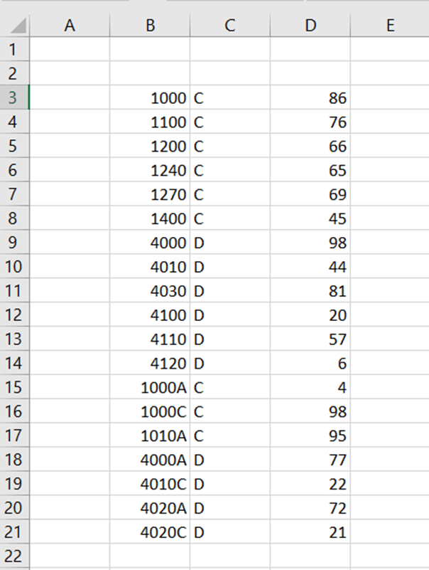
You have an accounting report including account, debet/credit and balance. A part of accounts are with four digits, a part with five. We should calculate total debit and total credit for accounts with five digits.
I tried with SUMIFS without success. Accounts with five digits are including letters, so the numeric condition would not work.
Luckily, SUMPRODUCT did not let us down.
The sentences are here:
=SUMPRODUCT((LEN(B3:B21)=5)*(C3:C21=G3)*D3:D21)
=SUMPRODUCT((LEN(B3:B21)=5)*(C3:C21=G4)*D3:D21)
First, we need to define that we are looking for values with five digits in column B. In column C, we are interested in values in G3 or in G4. After the sentence needs sum-column. Arguments are separated with multiplication sign.
The same data can be entered in MS Access.
The SQL query is:
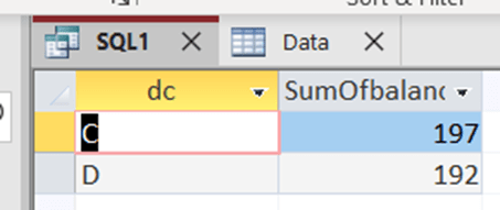
SELECT data.dc, Sum(data.balance) AS SumOfbalance
FROM data
WHERE account LIKE ‘?????’
GROUP BY data.dc;
Access return the same results as Excel.
Five digits in MS Access SQL is ‘?????’, two apostrophes and five question marks inbetween.
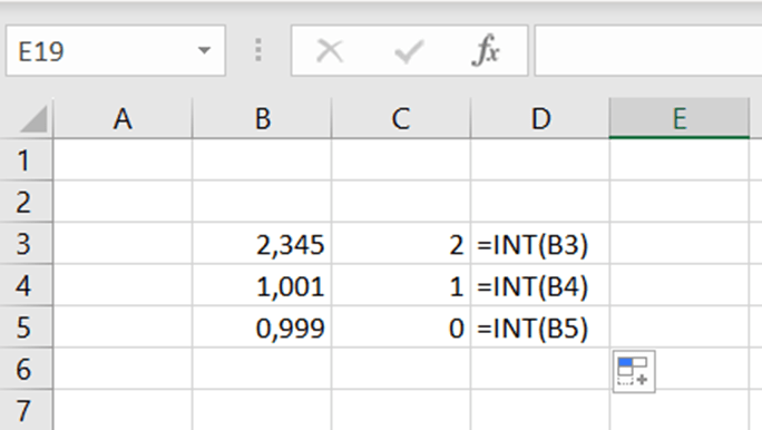
Do you know INT function ? It returns the integer or whole number.
This is not so complex.
In a park place, parking is free for the first two hours, after that parking costs two euros per beginning hour. Two hours and one minute parking costs two euros, two hours and 59 minutes costs two euros.
How to count this in Excel ?
The sentence is: =IF(B2<2;0;IF(B2-2>INT(B2-2);INT(B2-2)*2+2;(B2-2)*2))
If parking takes less than two hours, the fee is zero.
If the value minus two is higher than integer, meaning that there are decimals, then IF takes the integer value minus two and multiplies by two and adds two. If the value is not higher than integer, then value minus two is multiplied by two.
If we have value 4,1 – 2, that is higher than INT(4,1-2) which is two. Then we take integer (4-2) that is two multiplied by two and finally add two. That is six. If the value is sharp four, then just multiply four minus two by two, that is four.
If someone enters a negative value, the sentence returns zero. The input value is less than 2. Parking time cannot be negative but sentence was tested this way.
In case you prefer own functions, the respective code is here:
Function z_park2(hrs)
If hrs < 2 Then
z_park2 = 0
ElseIf (hrs – 2) > Int(hrs – 2) Then
z_park2 = Int(hrs – 2) * 2 + 2
Else
z_park2 = (hrs – 2) * 2
End If
End Function
The function returns the z_park2 value, which counted with input value hrs. If hrs is less than two, then z_part value is zero. If input value minus two is higher than integer for hrs minus two, then integer for input value minus two is multiplied by two and add two. If input value minus two is same as integer value minus two , meaning there is no decimals, then input value minus two is multiplied by two.
INT function in Visual Basic is similar than in Excel.
The input value needs to be in decimal format. Unfortunately, hh:mm format does not yet work.
As I started with, INT is not so complex function. Still, it nice to find how to use even simple functions. On the other hand, it is nice to make Excel count something which you could count mentally.
In this blog, I demonstrate four ways to calculate moving averages in Excel: with AVERAGE function, using data analysis, with OFFSET function, and adding moving average as trendline in a graph.
You can count manually the moving average. In the cell B6 we count average A2:A6. In the following the cell B7 the average is counted from A3:A7 and so on.
Another way is to install analysis toolpak in Excel option.
Then select data – data analysis – moving average.
Toolpak include different kinds of tools, but we are concentrating only on moving average.
Input range is the data range. Interval is five, we are taking average for five values. Output range is in B-column next to the values.
Press ok.
Excel created the averages automatically. As interval is five, first four values cannot have averages.
The moving average can also be done with OFFSET function.
In B6, we have an OFFSET function which has the reference in A2, then we do not move anywhere from A2 but just take five steps downwards. Then we activated area A2:A6. The nested function is taking AVERAGE from A2:A6. In the cell, we have a reference in A3 and function works fine.
This way is somewhat complicated but returns the same values as other options.
You can also add moving average into a graph.
Activate the data range and take insert – the graph.
Activate the line and take right mouse button, then select add trendline.
Select moving average and period 5.
As default the average line is quite thin, you can add value in width parameter.
You have sales values per day. You need to calculate the sum from last five days. When new values are added, the Excel needs to count only the five last values.
For example, if data is this:
2
3
4
5
6
2
the result is 20 (=3+4+5+6+2).
For the data
2
3
4
5
6
2
1
The result is 18 (=4+5+6+2+1).
First, we need ROW function.
The function returns the row number of the chosen value. A5 is in the fifth row.
We need to find the highest value for ROW function to find the last value in the array.
That we can do with the following statement:
=MAX(IF(A:A=””;;ROW(A:A)))
We are looking for the highest value, we need MAX function. If value in A-column is empty, the MAX should ignore that, if the value is not empty, then MAX is looking for the highest value in A-column. As we did not specify range, but stated just A:A, is the range whole A-column.
Now we should count the sum from rows 5 to row 9. For the step, we need OFFSET function, which I have covered in my earlier blog postings.
Offset-function consists of following arguments:
Reference. Where is the starting point of the formula ? That is always A1 as there is the first value of the array.
Rows. How many steps the formula takes downwards from starting point. We have nine values in the array and last five should be counted, the starting point is the row 5. OFFSET is taking four steps downwards.
Columns. How many steps the formula takes to the right from A5. We have all the values in one column, the value is therefore zero.
Height: How high is the area starting from A5. Five means the area of A5:A9.
The OFFSET is activating the range A5:A9, nested function SUM is summing the range.
The next step is to change static values into dynamic values.
The arguments are:
Reference is always A1.
Rows. Number of rows is counted as the highest row number in the range minus C4, which is five. Maximum row number is nine, that minus five equals to four. If you would like to sum for example four last values, change C4 to four.
Columns. No need to have other columns, value is always zero in our case.
Height: The range is five last numbers from C3.
Let’s do a test to see that the sentence is working.
You have a set of data. Duplicate values should be removed, so that only unique values are left. This can be done in multiple ways.
ID Product
1 A
2 A
3 B
4 O
5 O
6 U
7 U
8 U
9 W
10 K
11 A
12 S
We have a simple data running number (ID) and list of products. We should remove the duplicates and just see each different product once.
Data – data tools – remove duplicates
Maybe the most common way is to use remove duplicate functionality. Activate the data and press duplicate functionality button.
Press ok.
The duplicates were removed, and unique values are left in the list. As you noted, the functionality is overwriting the data. If you use this way, take a copy from the data and use remove duplicates for your copied data. Then you have originals untouched.
Here unique means that the product is listed just once. For example, A appears three times, there A is not unique. My thinking is that, if we take unique values, we take all the product listed just once. For example, product A is also listed and in unique values A is listed just once. Out of 12 values, we have seven unique values. According to conditional formatting, only four are unique.
This is a good way if you don’t want to change the data but just visualize the duplicates.
UNIQUE function
Write the UNIQUE and select the data, press enter.
The advantage with UNIQUE is that your original data and unique values are neatly separated.
COUNTIF function
Write in C2 =COUNTIF($B$2:B2;B2) and copy the formula downwards till C13. When the formula hits the first A in B2 the formula checks how many A letters are in B2:B2, and there is just one. In B3 the formula hits A again. Now the formula checks As in B2:B3, the formula returns 2.
Filter only number ones, and you have removed the duplicates.
You can also use Access to remove the duplicates.
The table consists of two columns running number ID and the product values. Data is similar than in Excel.
Create query at create – queries – query design.
Press property sheet.
You need to select unique values as “yes”.
Then drag the table to the middle of the screen.
Double click product field.
Run with exclamation mark. You get the results, seven unique values.
If you want to load the data from Access to Excel, select external data – export – Excel.
You can see the SQL, too. Select view- SQL view in query design.
As you noticed, we have many ways to find unique values and remove duplicates. Most often, I have used the first option, remove duplicates functionality. Also UNIQUE function is handy.
Standard deviation can be a useful function also in accounting and reporting. In case you want to compare some reports are sales steady or are the sales fluctuating.
Earlier Excel had a function STDEV, but that does not exist anymore.
Let’s calculate standard deviation manually.
We have values in column B. In column C we have average from column B. Column D indicates squared difference between the values and average. Sum of squared values equals to 24. 24 is divided either by number of values, in our case ten, or number of values minus one, nine. If you count the standard deviation for the sample we minus one from the count of values. When calculated for the population we divided by count of values.
Then you would get values 3 or 3,428571. Finally, you need to take square root from the number 3 or 3,428571. Square root from 3 is appr. 1,732 and from 3,428571 square root is 1,852.
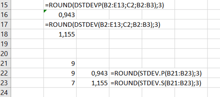
Here the different standard deviation formulas have been used with the demo data.
Looks like STDEV.P and STDEVPA return the same value for the population. Also, STDEV.S and STDEVA return the same value for the sample.
All the formulas have just one array. They are rounded into three decimals.
DSTDEV is more complex to calculate the standard deviation from a matrix.
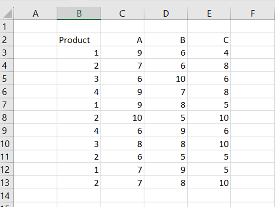
You have a sales report out of four products from one to four and out of three sales regions A, B, and C.
Then you would like to count the standard deviation for the product one in sales region A.
DSTDEV includes three arguments.
Database: the data area B2:E13.
Field: which sales area is investigated A, C2.
Criteria: which product is investigated 1, B2:B3.
The product 1 has been sold three times in sales region A twice nine pieces and once seven pieces.
The results have been rounded into three decimals.
DSTDEV is for sample and DSTDEVP for population.
How about if you wanted to know the standard deviation for the product 2 in sales region A ? If you select criteria B2:B4, then the function calculates the standard deviation for both products 1 and 2 in sales area A.
If you are handling values both with and without value added tax (=VAT), you occasionally need to split values with VAT to values without VAT and VAT itself.
For example, 100 includes VAT 24 %. The value without VAT is 80,65 and VAT 19,35. We are working with two decimals.
Values are counted this way: 0,24/1,24*100 = 19,35 and 1/1,24 * 100 = 80,65.
You can calculate this way.
If you are repeating this process frequently, you might want to create your own formula. Also rounding to two decimals could be added into the formula.
Write these formulas in Visual Basic editor. Functions are returning value for z_vat or z_vatzero with two input values sum and per. Sum is the sum with VAT and per is VAT percent.
Round function is used to limit the decimals to two. With Application.WorksheetFunction you can use normal Excel function in VBA.
Save the functions under personal workbook to have functions in use in all the Excel workbooks.
When writing a function, select fx insert function icon.
Select a category user defined function.
You can still double check. 80,65 * 0,24 =19,35.
As said, only input parameters are the sum and the percentage. The result of user defined function is already rounded.
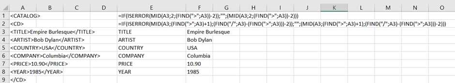
Or even better to have name of the segment and data itself in separate columns like this:
TITLE Empire Burlesque
ARTIST Bob Dylan
COUNTRY USA
COMPANY Columbia
PRICE 10.90
YEAR 1985
To extract the data, we can use MID function which extract several characters from the middle of the string.
MID consists of three arguments:
Text: from which text MID is extracting characters.
Start_num: what is the first character to be extracted.
Num_char: how many characters are to be extracted.
To extract the segment, can be done with following sentence MID(A3;2;(FIND(“>”;A3))-2.
The extraction is in cell A3, we are starting from the second character. The number of characters is defined with FIND formula. FIND is looking for the > sign. > is the 7th character, we need to deduct two from the result. We take five digits starting from second character.
<TITLE>Empire Burlesque</TITLE>
In case the MID returns an error value, we rather have an empty value than an error.
The sentence to return the data content is more complex.
The first argument, text, is easy. We have the text in A3 cell. The start number is where > is added by one.
<TITLE>Empire Burlesque</TITLE>
In XML above, the data starts with 8th character.
Number of characters is calculated by finding where / sign. That result is deducted by where > situates. That result is deducted by two. In Empire Burlesque example the / is 25th character, > is the seventh. 25 minus seven minus two equals 16. The MID needs to extract 16 characters starting with eighth digit as / is the seventh digit and we need to start extracting from the following character.
Just one notification, there are two > signs in the string. FIND function holds the argument start_num, where the find starts. As that is not defined, the FIND returns the value for the first >, which is something we are looking for.
You have a sample data about persons. The data includes also birth year. We should investigate what can we find out about age distribution. The data is imaginative, and the data can be found at the end of this blog.
We need to group the data like how many persons are born in which decade and create a graph. How many persons are born in 1940s and how many in 1950s and so on.
Count all the persons whose birth year is 1940-1949 to get the number for 1940 bucket. We need to count how many persons are born in 1940 or later. Then we minus how many persons are born in 1950 or later. The result is the persons born in 1940s.
For example, there are 85 persons persons born in 1950 or later and 67 persons born in 1960 or later. Therefore, we have 18 persons born in 1950s.
For the first the value we need to count all the values minus the values higher or equal than 1940.
The COUNTIF function holds arguments range and criteria. First we define range like C3:C104 where the values are and then the criteria when the value in range is equal or greater than the value in the cell F5. To define equal or greater than F5, we use the phrase “>=”&(F5). COUNT simply counts how many times the criteria is fulfilled.
To create a graph, activate the range F3:G14. Leave the cell F3 empty but populate the G3.
Then select insert and choose graph.
The graph:
Now we have visualized the data.
We can see, that the first peak is from those who were born in 1940s and 1950s. Second peak is from 1970s and 1980s. The last peak is from 2010s. It looks like the sample includes three generations. The first generation is from 40s and 50s, their descendants were born in 70s and 80s. The third generation was typically born in 2010s. The clearest and most obvious peak is in 2010s. The second clearest is the first generation. We have only few observations from 1990s and 2000s.
You have a simple VLOOKUP, but somehow it does not work. Even though VLOOKUP is correctly written. This might depend on several things.
VLOOKUP is looking for qw34 value in the range (B3:C5). Then one column right from qw34 is selected. The expected value is 1, but the VLOOKUP does not return that value.
As said, this might depend on several things. In our case, there are invisible spaces after qw34 in the cell of B3. This can be found with LEN function. LEN return the number of characters in a string, invisible spaces are counted and increasing the length.
The VLOOKUP does not return 1 as the value in B3 is “qw34 ” with six characters and the value in F3 is “qw34” with four characters. VLOOKUP does not simply find “qw34” in B3:B5.
We can correct with TRIM function, which is removing spaces.
To do this easiest way, we can execute Visual Basic code to manipulate the cells with TRIM.
Sub z_vlookup_trim()
Dim za, zn
Do
za = ActiveCell.Value
zn = Application.WorksheetFunction.Trim(za)
ActiveCell.Value = zn
ActiveCell.Offset(1, 0).Select
Loop Until ActiveCell = “”
End Sub
First, the variables za and zn are introduced. The variable za is receiving the value from the active cell. If you execute the macro when the cell B3 is activated, then za gets the value “qw34 ”. The variable zn is za manipulated with Excel function TRIM. The value for zn is “qw34”. The VBA proceeds downwards till the active cell is empty.
Place the cursor in B3 and execute the macro.
After the macro has been executed, the TRIM has trimmed the B3:B5 area from spaces. VLOOKUP in G3 finds the value one. One benefit using a macro is that we don’t have to add any new values in a worksheet.
The expression Application.WorksheetFunction. is a useful way to call an Excel function inside VBA macro.
In an earlier blog, I have introduced SWITCH function to replace IF. Then a condition was for an exact value, like switch “P1” value to “Jan”.
Now we have bit different SWITCH case. If the value is less than 10, then the returned value is “small”, if the value is from 11 to 14, then returned value is “mid”, the values from 15 to 19 are “fair”, and above, the returned value is “large”.
Earlier, the first argument in SWITCH was cell where the value is, like C4 in our case. However, when we don’t have exact values but less than operator, the first argument is TRUE. Then we have condition if C4 is less than 10, then the returned value is “small”. If C4 is less than 15, then the sentence returns value “mid”. In case C4 value ranges from 15 to 19, then SWITCH returns “fair”. For value 20 and above, the returned value is “large”.
Let’s check a case where we have two input parameters and need to evaluate combination of the two parameters.
Column C may have values 1 or 2, column D may have values a or b. If C equals to 1 and D equals to a, the result is one a. When C is 1 and d is b, the outcome is one b. If C equals to 2 and D a, then result is two a. In case C is 2 and D is b, then the right value is two b.
The key is that for value, we need to combine B4 and C4. Like when combination of B4 and C4 equals to 1a, then the result is one a. Just remember to write value inside parenthesis. Similarly, define all the four combination and the wanted result.
Both IF and SWITCH returned correct values. Still, I prefer SWITCH as we need IF several times and then we need also several parenthesis. When writing a SWITCH sentence, it is easier to have one block in clipboard, paste the block and modify it.
Maven Analytics published data sets about pizza sales in their website Free Data Sets & Dataset Samples | Maven Analytics . Thanks for Maven for providing data for training purposes. In this blog I am analyzing the data and answering the four questions in Maven web site.
The data was downloaded into MS Access. As Access is a database, then the data was in a database where we can browse the data with SQL.
Order details includes data about orders, which pizza was ordered and how many pieces. There are close to 49k records in the table.
Order table has the order date and time. Order_id is the primary key field.
Pizza_types
The primary key in this table is the first column, pizza_type_id. In the original data, the ingredients were in one column. I have separated the ingredients in different columns.
The pizza_type table holds the prices and sizes of each pizza. The pizza_type_id is a higher level parameter. Each pizza_type_id is divided into normally three pizza_id depending on the size.
Unfortunately, the decimals were dropped from prices. Therefore my price estimates are bit lower than real figures, but I am not that far from real figures.
The date table is an additional table which is not part of an original data set. I will use date table in reporting, as we want to know eg. sales per each weekday.
The data was loaded into Excel data model.
In date table, month, week of the year, day name, and month were added.
In Power Query a new column “hour” was added to orders table. We can use this calculated column for defining peak hours.
This is the data model how tables are related to each other.
Here are the relations.
Both order_details and orders tables have order_id field. Order_detail table holds the order id, pizza id and quantity. orders table includes the ordering time. The cardinality is many to one, order_details table is per pizza and one order may include several pizzas, one order has just one order time.
Pizzas is a pizza master data table. Order_details include which pizzas have been ordered. As said, one order my include several pizzas. Therefore each pizza needs to exist just once in master data table, before you can order the pizzas. The cardinality is one to many.
Orders table has the ordering date. The relation is created to date table. One date may exist several times in orders table, as many orders may be placed during one day. Each date from the year 2015 exists once in data table.
All the pizzas are listed in pizzas table, as the pizza_types table consists of ingredients of different pizzas. Pizza_type_id is the same field in both tables. In pizza_types table pizza_type exists just once, as pizza_type is primary key in pizza_type table. In pizzas table the pizza_type_id may exist several times, as pizza_id is the primary key .
How many customers do we have each day? Are there any peak hours?
There are altogether 21350 orders during the year 2015. This means we have on average 58 customers a day, when we count one order as one customer. Busiest day was Nov 27th. Then we had 115 customer. Lowest number of customers, 27, was seen in Dec 29th.
We can see two peak hours. First peak takes place between 12-13, obviously customers are having lunch time. Another peak is during dinner time 17-18.
How many pizzas are typically in an order? Do we have any bestsellers?
Average number of pizzas per order is 2,3. Highest number of pizzas in one order is 28 pizzas.
The best selling pizzas are: classic_dlx, bbq_ckn and Hawaiian.
How much money did we make this year? Can we identify any seasonality in the sales?
My answer for total revenue is 795200.
The revenue was calculated with the formula below. However, when transferring the data from MS Access to Excel data model, I lost he decimals in prices. This means, my revenue is slightly lower than the correct amount.
The best pizza, in financial terms, is The Thai Chicken Pizza.
The total revenue was checked also in Access.
The result is the same.
SELECT SUM(order_details.quantity * pizzas.price)
FROM order_details INNER JOIN pizzas ON order_details.pizza_id = pizzas.pizza_id;
This is the SQL statement to query the total revenue.
About seasonality in sales:
When checking orders volumewise, meaning counting number of pizzas, the best month is July followed by May. The best weekday for pizza selling is clearly Friday. Saturday and Thursday are second best days, Saturday and Thursday have nearly equal sales but evidently lower than Friday.
Are there any pizzas we should take of the menu, or any promotions we could leverage?
Mushroom is the least popular.
The other four categories are quite equally popular, but mushroom is an exception. Would it be a good idea to remove mushroom from menu ?
There are practically no sales before 11 o’clock. Some promotion could take place to balance the workload more evenly throughout the work day.
About the pizza sizes, S, M, and L cover nearly 99 % of all the sales. XL and XXL have portion of good 1 % out of total sales. Should the XL and XXL be removed from selection or should they be promoted ? At a moment XL and XXL do not have significance in pizza business.
You have sales data with dates. When you take reports, we are not interested in dates but rather sales per month and year.
The columns are product, sales date, and sales volume.
We would like to know what the sales would have been for product a in Nov 2019 ?
Easiest way is to add extra columns to define year and month.
The column E is populated with MONTH formula and F with YEAR.
The November 2019 sales for product A can be counted this way.
First argument is sum column, which means column C as we have there the sales volume. Then we show where the product data situates, that is column A. Then the product we are interested is a in the cell I2. The range for month is in E column and the month value in J2. Similarly, the years are in F-column and year criteria in K2.
During Nov 2019 altogether 12 pieces of product ‘a’ were sold.
Another option is to use SUMPRODUCT function. The product information is in A-column, criteria which product is searched for is in F4. The dates are in B column, the criteria is in G4 inside the MONTH formula and the criteria for year in H4. Finally, sum column is in C2:C13. The arguments are separated by multiplication sign.
For me, SUMPRODUCT is more compact than SUMIF. With SUMIF you need to add extra columns. If you handle large data sets, make new calculated columns the data even larger. As with SUMPRODUCT, you can embed month and year formulas inside SUMPRODUCT.
Just for comparison, I downloaded the same data into MySQL table.
You have sales data scattered in several tables. Structure is not same from table to table.
The first table has columns ID, product, and sales volume. The second table has columns ID, product, region, and sales volume. The third table has columns ID, product, region, sales representative and sales volume.
Product and sales volume can be found in all the three tables. We can create a report to count sales volume per product throughout the three tables.
Table 1.
Table 2.
Table 3.
Load the tables into data model.
Take the menu path data – get data – combine queries – append.
Append means that we are building a table on top of another.
Inculde all the three tables.
For the tables without values in region or sales rep fields, the Excel enters “null”. Region and sales rep fields cannot be used as the fields are not in every table. The common table is named as T1T2T3.
Create a pivot on top of data model.
Create a simple SUM formula.
Pivot settings.
The results.
One way is to check with SQL in MS Access.
SQL is here:
SELECT product, SUM(sales)
FROM (SELECT product, sales
FROM t1
UNION ALL
SELECT product, sales
FROM t2
UNION ALL
SELECT product, sales
FROM t3
) AS t
GROUP BY product;
If you don’t need grouping by product but you would like to see just the total number. In that case just remove the GROUP BY line, and product in SELECT statements.
If you have data bit scattered between several tables, but if the tables have common fields, it is possible to sum up the columns.
You have a sales report with sales value and a dimension. Normally, you calculate certain dimensions like a, b and c equals to something. Like how much is the total sales for dimensions a, b, and c.
A, b, and c dimensions can be calculated with following sentence:
First SUMIF counts the totals for dimension a, second for b, and third one for c. After that all the SUMIFs are summed together. The formula returns the value 36.
If you need to exclude dimensions ? You should calculate other dimensions than a, b, and c. What is the sales volume for other dimensions than a, b, and c? One way is to calculate the total and then minus the sentence above.
First you need to show the values in B2:B11, then dimensions C2:C11 and which dimension are we looking for not equal to a, not equal to b, and not equal to c.
Another way to calculate other dimensions than a, b and c:
You have a sales report and you need to count an average. That’s easy. However, there is one exceptionally high value in the report. That is not a normal value, therefore the average is higher when all the values are counted than without one high sales figure.
One option is to exclude extreme values in the bottom and in the top. The very high sales value will not be counted but also the low values are not considered, either.
Instead of AVERAGE function use TRIMMEAN.
Here is a sales report. As you can see, the last value is considerably higher than other values.
The average for this report is 61.
We would like to exclude lowest and highest 10 % from the report, then the 200 value would not be counted. The old PERCENTILE function does not exist anymore, now we have PERCENTILE.INC and PERCENTILE.EXC. Both the functions have two arguments: array and percentile. If we want the lowest 10 %, then the percentile is 0,1. For the highest 10 %, the percentile is 0,9.
The results with percentile. Exc takes wider values than inc.
Let’s mark manually the values with ‘X’ in the middle when top 10 % and low 10 % are excluded.
The formula in C3 is =IF(AND(B3>$F$3;B3<$F$4);”X”;””). B3 needs to be higher than F3 and lower than F4. Then the value is in the middle and marked with X, not in top 10 % or top low 10 %.
Now, if we calculate the average for the values with X and then TRIMMEAN for the data range, then values should be codirectional.
The average for X marked values are counted in C1 =AVERAGE(IF(C3:C24=”X”;B3:B24)).
Write the sentence and press shift+control+enter not just enter. After pressings shift+control+enter Excel adds arch brackets.
The sentence in D1 is =TRIMMEAN(B3:B24;0,1) . Simply, what is the data range, and what is the percentile. What is proportion of excluded values in data range. In our case it is 0,1, meaning that 10 % should be excluded from top and from bottom.
Both manual average of selected values, marked with X, and TRIMMEAN for data range count pretty similar numbers.
The average of 61 is slightly different than 56, when we excluded exceptionally high and low values. TRIMMEAN is a useful function also in reporting.
SWITCH function is quite straightforward. First you need to define the cell where is the value. That is B3 in our case. Then you specify if the value is like P1, then which value the function should return, that is Jan. If the value is P2, then SWITCH returns Feb. Please, note that when B3 is once defined, we don’t have to repeat the cell address.
One benefit with SWITCH is that you don’t have to count parentheses.
It is easier to nest the SWITCH than IF above.
Say, you have month and year as P5/21 meaning May 2021. This should be changed to May/21. The SWITCH above is not enough.
First, we need to extract P5. The slash might be third or fourth digit. This we can do with IF-formula below.
If slash is the third digit, then two first digits are selected. If slash is the fourth digit, then three first digits are selected. From P5/21, only P5 is returned.
Here we combine the IF which is taking the P5 from P5/21. Then SWITCH is switching P5 to May. Finally, three last digits in E3 are added at the end of F3.
Think if you still had IF instead of SWITCH, the sentence would be even more complex. With SWITCH the sentence is clearer to comprehend. SWITCH makes possible to build longer sentences easier than IF, that is my opinion.
You have set of reports, the structure is not identical throughout the reports. Let’s see what Excel consolidation can do.
Icon for consolidation can be found under data menu, and top right-hand corner in data tools section.
We have sales reports from three regions North, South and East. Each of region consists of four sales representatives who are selling trucks, vans and automobiles. The reports have two dimensions.
Report from South.
Report from North.
Report from East.
As you noticed, the files have been named according to the geographical region.
Sales rep Jeremy works only in East region replacing Jack. He works in South and North.
Open the consolidation Excel sheet and press the consolidation icon.
The consolidate box appears. I placed the cursor in B2 cell in each of the reports.
The function is SUM as we are summing up all the three regions.
I activate all the three parameters under “Use labels in”.
I pressed the arrow up at the end of the reference window and consolidate -reference window opens.
Just open the first report and activate the data range. Press enter.
Press add.
The reference is moved to all references window.
Empty reference window and press the arrow at the right-hand side of the window.
Browse the data range in the next report and press enter.
Again, press add.
Empty the reference window and press the arrow up.
Browse the data range from the last report and press enter.
Add the last data range into the all references window.
Empty the reference window and press ok.
This report appeared in the consolidation Excel. The main window includes sales reps and product categories. The regions are not visible.
If you press number two in left-hand side margin. Then the region-specific division appears. Note that the product line, like trucks, is the sum line. For example, Jill was selling three trucks in all the three regions. The Excel correctly calculates the different sales reps.
Consolidation might be handy sometimes, if you combine data tables which are not totally equal. A benefit with consolidation in Excel, is that it is easy to take into use. It does not take long time to comprehend the feature.