Substituting Scandinavian letters

You might have faced the issue that the system does not understand Scandinavian letters ä, ö or å. Instead, the normal a or o should be written instead of ä, ö or å. This will happen with email addresses. I will show an example of emails bit later.

Yrjö Pyykkönen should be written as Yrjo Pyykkonen.

This we can tackle with SUBSTITUTE function.

The function consists of three main arguments: the text where substitution is done, the value to be substituted and the value to substitute.

In this case, we are checking the value in B3 cell. If there are any “ö” letters, those are substituted by “o”.

This does not substitute capital letters, like “Ö”.

Only minor ö was substituted.

However, we can create a nested SUBSTITUTE.

The sentence in D3 is =SUBSTITUTE(SUBSTITUTE(B3;”ö”;”o”);”Ö”;”O”).

If you want to substitute “å” and “ä” to “a”, and “ö” to “o”, both capital and small letters, then the sentence is:

=SUBSTITUTE(SUBSTITUTE(SUBSTITUTE(SUBSTITUTE(SUBSTITUTE(SUBSTITUTE(H3;”Ä”;”A”);”Å”;”A”);”Ö”;”O”);”ä”;”a”);”å”;”a”);”ö”;”o”)

Let’s see how the sentence works in practice.

Fill the first name and the last name. Then create an email address for the person.

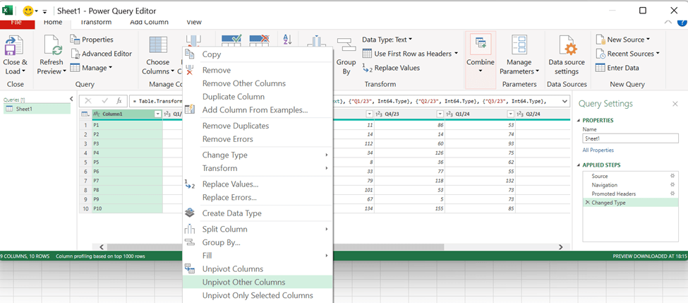
Select data – flash fill (under data tools).

AI based functionality is creating the email address for all the names based on the model for the first name. This is supervised learning for AI.

Looks good, but Åke Sandström has Scandinavian letters in the email. Scandinavian letters should not be in the email.

The sentence in the cell E3 is =SUBSTITUTE(SUBSTITUTE(SUBSTITUTE(SUBSTITUTE(SUBSTITUTE(SUBSTITUTE(B3;”Ä”;”A”);”Å”;”A”);”Ö”;”O”);”ä”;”a”);”å”;”a”);”ö”;”o”)

After the Scandinavian letters have been substituted, the emails can be created based on names without Scandinavian letters.

Pivot format

We have a sales report about products P1 to P10 by quarters from Q1/23 to Q4/24.

Which of the following products saw the largest increase in sales from 2023 to 2024 ?

We can calculate manually the sums for 2023 and 2024 and calculate the change between the years. Sales for P5 have increased mostly when measure the relative change.  

This way we need manual adjustments. We could make a data model and count with DAX.

The data is not in pivot format. The data should include fields product, quarter and sales volume. The data should not be in matrix format.

Download the data into Power Query, activate the first column and then select right mouse button and unpivot other columns.

Now the data is in Pivot format. Add the column headers.

The power query data is loaded into data model. Each row contains product, quarter and sales volume.

Choose close & load to…

Select only create connection and activate add this data to the data model.

Now we have the same data but on top of the data model.

We need the formulas to calculate the year total with DAX.

SUM23 = CALCULATE(SUM(Pivot2[Sales]);Pivot2[Quarter] IN {“Q1/23″;”Q2/23″;”Q3/23″;”Q4/23”})

SUM23 sums the quarters from 2023.

Pivot2 is the table. Sales is the field for sales volumes. Quarter is the time field. Q1/23, Q2/23 and so on are the values in quarter field.

The same pattern works for the total sales in 2024:

SUM24 = CALCULATE(SUM(Pivot2[Sales]);Pivot2[Quarter] IN {“Q1/24″;”Q2/24″;”Q3/24″;”Q4/24”})

Finally, we calculated the change between the years.

Change = ([SUM24]-[SUM23])/[SUM23]

Sales for P5 increased most between 2023 and 2024 compared to other products.

We have the same results but with less manual work. We have the data in data model and DAX was calculating the results. The benefit with data model is, that we can create other measures with DAX on top of the data model.