Mode is the value which appears most in data range. For example, in the data range 1, 2, 2, 3 and 4. The mode is two as it exists twice, but all the other numbers exist only once in the data range. Number two has the highest frequency.

Mode is easy to calculate with Excel. Just take the MODE function, the only argument is the data range.

If we have multiple modes in our data range. Both two and four are modes. Still, MODE takes just the first mode. It is true that two is mode but MODE neglects another mode, four.

We have an Excel function MODE.MULT which returns multiple values if there are more than one mode. I wrote the sentence in the cell D2 and pressed enter. Excel automatically populated cells D2 and D3.

MODE.MULT is useful as you never know if there is more than one mode in data range.

One thing to note, as MODE.MULT might populate several cells downwards, it is useful to leave some cells empty below the MODE.MULT.

I was calculating the average in D3 cell. After that, I entered MODE.MULT in D2.

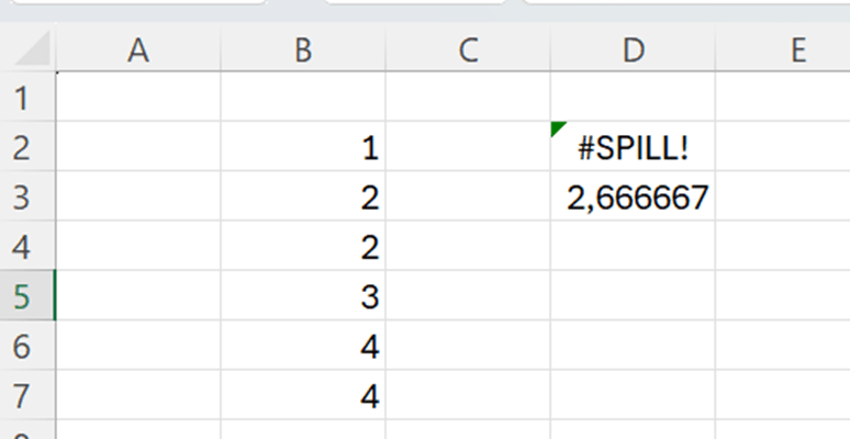
When I pressed enter, this is the result.

Better to do another way round, first average which is taking for sure just one cell. After that enter MODE.MULT.  

The function MODE.SNGL, but that works as MODE.

If you ever need to count which value has the highest frequency in your data range, I recommend you use MODE.MULT. Especially, if you deal with large data sets, and you cannot know whether there are several modes in the data set. Just prepare few cells below the sentence, if MODE.MULT returns several values beneath the sentence.