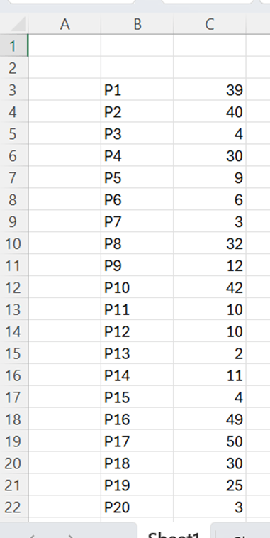
You have a sales report about twenty products. You need to classify them into four categories based on the sales. A controller may then check the products in the lowest category.

Here we can use QUARTILE formula. Quartile means that we divide the data range into four groups each of them including one fourth of all the values.

So, the controller wants to concentrate on the fourth selling least.

We need to define in the lowest quarter which products have the lowest sales.

To divide data range to quarters happens easily with QUARTILE.EXC function.

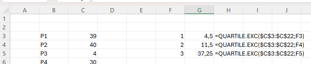
The quartile limits are 4,5; 11,5 and 37,25. The function defines just three values as the fourth one is higher than 37,25.

How many product have been selling less than 4,5 ?

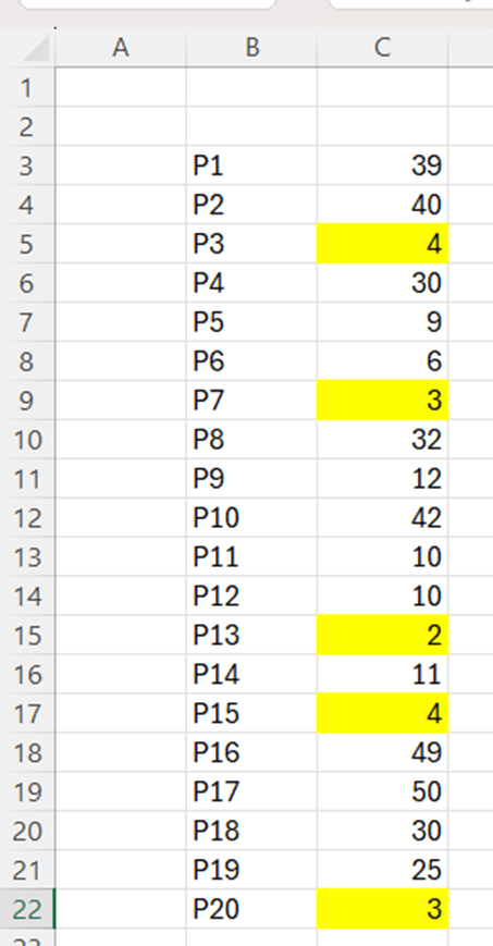
We have five product with sales less than 4,5. It would be better if we had a number next to sales representing into which quartile the product belongs. The higher number means higher sales and higher category.

This is the sentence in D4: =IF(C3<=$G$3;1;IF(C3<=$G$4;2;IF(C3<=$G$5;3;4))).

If C3 value is equal or lower than G3, then the value is one. If C3 value is equal or lower than G4, then the value is two. If C3 value is equal or lower than G5, then then the value is 3. In any other cases, the value is 4.

Now the twenty products are divided into four groups, each of them containing five products. The controller may take a closer look at the category one.

Just to double check, we can still count that there are five products in all the categories.

Each of number from one to four appears five times.  Quarterly division works.

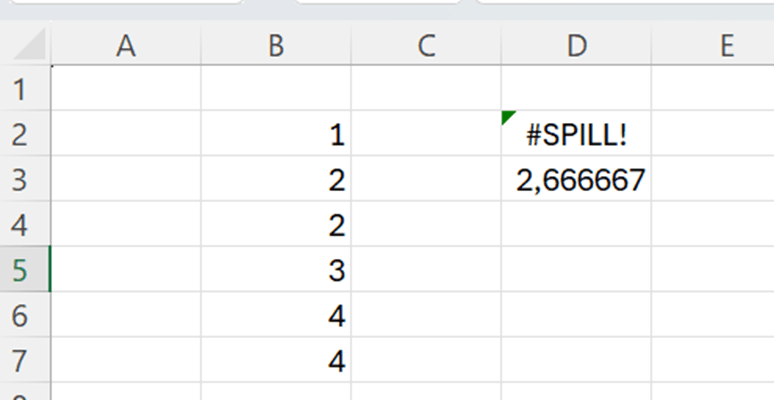
Another method to determine the five products with lowest sales, is to use RANK function. Here is a short introduction to RANK.

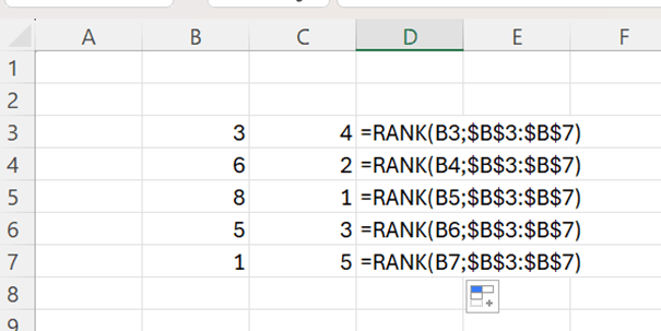
With RANK we are setting rank order for the values in B3:B7. 8 is the highest with value one, 6 is the second highest with two and so on.

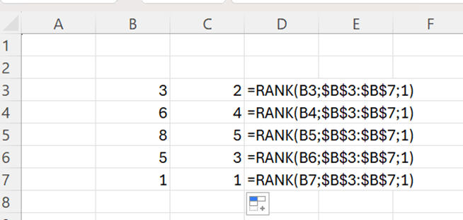
When I add one argument, the rank order is descending, the 8 is the highest with value 5.

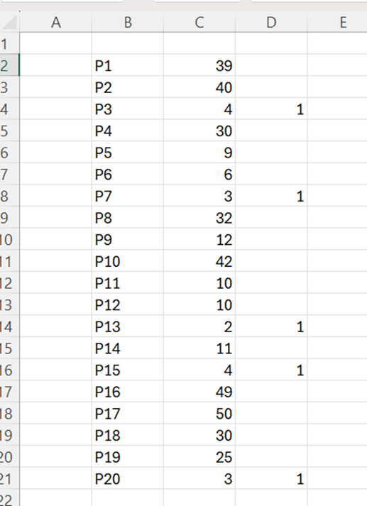
The sentence in D2 is =IF(RANK(C2;$C$2:$C$21;1)<=(COUNT($C$2:$C$21)/4);1;””).

If descending rank for the value C2:C21 is lower or equal than number of all the values in C2:C21 divided by four, then value is one. If statement is not true then value is empty.

Excel sets descending rank values for each cell, if the rank is five or less, then value is one, otherwise the value is zero.

This way we can also find five product with lowest sales.

Mode is the value which appears most in data range. For example, in the data range 1, 2, 2, 3 and 4. The mode is two as it exists twice, but all the other numbers exist only once in the data range. Number two has the highest frequency.

Mode is easy to calculate with Excel. Just take the MODE function, the only argument is the data range.

If we have multiple modes in our data range. Both two and four are modes. Still, MODE takes just the first mode. It is true that two is mode but MODE neglects another mode, four.

We have an Excel function MODE.MULT which returns multiple values if there are more than one mode. I wrote the sentence in the cell D2 and pressed enter. Excel automatically populated cells D2 and D3.

MODE.MULT is useful as you never know if there is more than one mode in data range.

One thing to note, as MODE.MULT might populate several cells downwards, it is useful to leave some cells empty below the MODE.MULT.

I was calculating the average in D3 cell. After that, I entered MODE.MULT in D2.

When I pressed enter, this is the result.

Better to do another way round, first average which is taking for sure just one cell. After that enter MODE.MULT.  

The function MODE.SNGL, but that works as MODE.

If you ever need to count which value has the highest frequency in your data range, I recommend you use MODE.MULT. Especially, if you deal with large data sets, and you cannot know whether there are several modes in the data set. Just prepare few cells below the sentence, if MODE.MULT returns several values beneath the sentence.