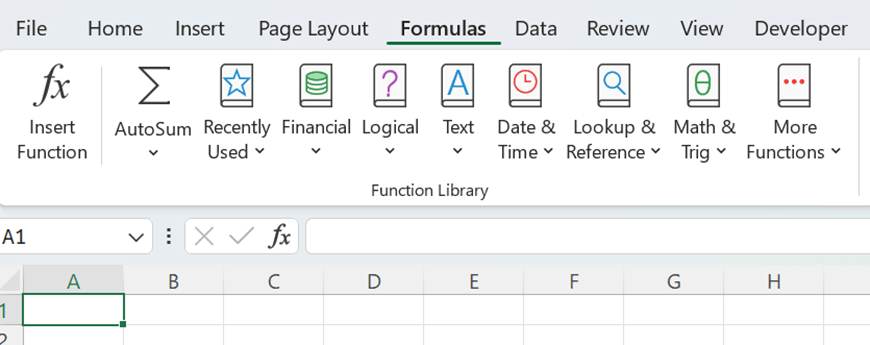
Have you checked how many different ready made formulas can be found under formulas menu ?
For example, these formulas are under logical section and there is still side bar that some functions are not visible.
I checked duration as I have studied some finance.
Duration means that if you invest in bonds, after how many years you will get back the money you invested in bonds.
You invest 100 € in bonds and you will get 3 % coupon interest annually, means 3 € a year. At the end of maturity 10 years, you will get both invested capital and coupon back 103 €. Market yield is 8 %.
The formula in F2 is =1/(1+$B$6)^D2, meaning 3/(1+1,08)^1. This means the cash flow is discounted with 8 % interest.
G2 has formula =E2*F2. That is the cash flow in present value. H2 has sentence =G2/SUM($G$2:$G$11). H2 calculates percentage of cash flows in present value per year. I2 is =D2*H2. This is year multiplied by percentage of cash flows in present value per year.
Finally, the values in (I2:11) are summed. That value is duration. The investor would get the money invested back in close to 8,5 years. If coupon interest is increased, the duration is decreased, as the investor gets the money back bit faster.
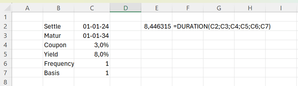
Let’s see how the standard DURATION function under financial functions works.
The arguments for the DURATION function are:
Settlement: start date of the bond.
Maturity: end date of the bond.
Coupon: annual interest rate for the bond.
Yield: discount percentage, the cash flow is discounted to present.
Frequency: how many times a year the coupon interest is paid.
Basis: how many days are in a year. This parameter does not affect much the formula, according to my testings.
The DURATION function returns the same value as value calculated manually. Of course, ready made function is faster and easier. Still, it is useful to understand how function is calculating the values.
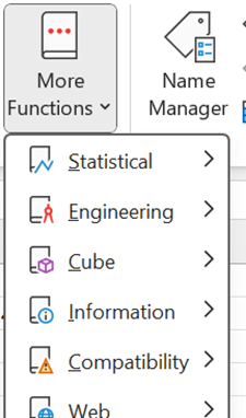
DURATION is just one example out of hundreds of formulas in Excel. You might find formulas suitable for your requirements and then you don’t have to enter all the values manually.
Standard deviation 1 = standard deviation of security 1
Portion 2 = percentage of security 2 in portfolio
Standard deviation 2 = standard deviation of security 2
Correlation = Correlation between security 1 and security 2
We have two securities in our portfolio, A and B. Expected return for A is 5 % and standard deviation is 8 %. Expected return for B is 15 % and standard deviation is 18 %. Security A is clearly a low-risk investment compared to security B. The mutual correlation is 12 %.
You can calculate standard deviation just like this:
=(C3^2*C5^2+2*C3*C5*D3*D5*C6+D3^2*D5^2)^0,5
If you calculate this repeatedly, it is useful to create your own function.
We are calculating the value for z_port. For that we need five input values p1, s1, p2, s2 and co.
Input arguments are:
P1 = percentage of security 1 in portfolio
S1 = standard deviation of security 1 i
P2 = percentage of security 2 in portfolio
S2 = standard deviation of security 2
Co = Correlation between security 1 and security 2
You need to enter five input arguments to calculate the standard deviation.
Let’s calculate also the expected return.
It is simple
P 1 = percentage of security 1 in portfolio
R 1 = expected return of security 1 i
P 2 = percentage of security 2 in portfolio
S 2 = expected return of security 2
The custom function would be:
Function z_ret(p1, r1, p2, r2)
z_ret = p1 * r1 + p2 * r2
End Function
Writing a custom function for expected return does not save so much time compared to calculating the same manually. Still, it is a neat presentation to have a custom function.
Both manual counting and custom functions return the same values.
We are investing in a two-security portfolio. Our investment policy is to be risk averse, meaning that we prefer to have a portfolio with as low risk as possible. We need to minimize the standard deviation. Intuitively, we should invest all the money in security A and nothing in security B.
In our case also the correlation plays a part as correlation is low, it means that we can effectively diversify risk by investing in both the securities.
When correlation is low, it is possible that when value of one security is decreasing, the value of another might be increasing. The total value of the portfolio would not decrease that much.
We have a matrix with proportions of A and B securities with an interval of 10 %. Then we have standard deviation and expected return with those proportions. We can see in the matrix that standard deviation is dropping a bit when we increase the proportion of security B in our portfolio.
The sentence in D11 is =z_port(B11;$C$5;C11;$D$5;$C$6) and in E11 =z_ret(B11;$C$4;C11;$D$4).
We draw a graph by selecting the data range. Just untick B in the left box as we want B to be horizontal axis. Press “edit” in the right box and select value 0%-100% under B.
We see in the graph that standard deviation is dropping slightly as we increase the proportion of security B in our two-security portfolio. Expected return is linear.
When we include more of security B in our portfolio, the expected return increases. The optimized portfolio is not only of lower risk but also the expected return is higher than investing everything in security A.
If you don’t have yet solver add-in in Excel, you can activate that in Excel options.
Then solver appeared under data ribbon. In my Excel it is in the furthest right corner.
We want to minimize the portfolio standard deviation I4 by changing the proportion of security B E4.
Solver found results.
If we invest 13 % in security B and 87 % in security A, we have the lowest risk level, minimum variance portfolio. Also, the expected return is more than 6 %, that is more than what we would expect by investing in security A only.
Now A and B are not correlating with each other much. Let’s change the calculation and increase the correlation to 60 %.
Solver is proposing to invest only in security A. There would not be diversification between A and B, but everything would be invested in A. Then the expected return is 5 %.
Let’s drop correction to negative -5 %.
18 % should be invested in security B, also expected return is higher than in earlier scenarios.
When correlation is slightly negative, the portfolio turns out to be more profitable with less risk.
The graph is drawn with the assumption that correction is – 5%. We can see from the graph that our portfolio is having lower standard deviation but higher profit.
If you invest in two different securities, it is better to choose the couple that correlates as less as possible with each other.
Another takeaway is the solver. If you need to find an optimal solution for some calculations, test the solver. We wanted to find the minimum value of one parameter by changing the other parameter.