SUM IF NOT

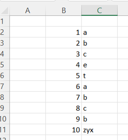
You have a sales report with sales value and a dimension. Normally, you calculate certain dimensions like a, b and c equals to something. Like how much is the total sales for dimensions a, b, and c.

A, b, and c dimensions can be calculated with following sentence:

=SUMIF(C2:C11;”a”;B2:B11)+SUMIF(C2:C11;”b”;B2:B11)+SUMIF(C2:C11;”c”;B2:B11)

First SUMIF counts the totals for dimension a, second for b, and third one for c. After that all the SUMIFs are summed together. The formula returns the value 36.

If you need to exclude dimensions ? You should calculate other dimensions than a, b, and c. What is the sales volume for other dimensions than a, b, and c? One way is to calculate the total and then minus the sentence above.

=SUM(B2:B11)-(SUMIF(C2:C11;”a”;B2:B11)+SUMIF(C2:C11;”b”;B2:B11)+SUMIF(C2:C11;”c”;B2:B11))

Using SUMIFS function, you can use the sentence below.

=SUMIFS(B2:B11;C2:C11;”<>a”;C2:C11;”<>b”;C2:C11;”<>c”)

First you need to show the values in B2:B11, then dimensions C2:C11 and which dimension are we looking for not equal to a, not equal to b, and not equal to c.

Another way to calculate other dimensions than a, b and c:

=SUMPRODUCT((B2:B11)*(C2:C11<>”a”)*(C2:C11<>”b”)*(C2:C11<>”c”))

The logic with arguments is somewhat similar to SUMIFS. First, you need to show values B2:B11 and then dimensions and which dimensions are excluded.

For me, both SUMIFS and SUMPRODUCT are simpler than SUM/SUMIF.

TRIMMEAN function in reporting

You have a sales report and you need to count an average. That’s easy. However, there is one exceptionally high value in the report. That is not a normal value, therefore the average is higher when all the values are counted than without one high sales figure.

One option is to exclude extreme values in the bottom and in the top. The very high sales value will not be counted but also the low values are not considered, either.

Instead of AVERAGE function use TRIMMEAN.

Here is a sales report. As you can see, the last value is considerably higher than other values.

The average for this report is 61.

We would like to exclude lowest and highest 10 % from the report, then the 200 value would not be counted. The old PERCENTILE function does not exist anymore, now we have PERCENTILE.INC and PERCENTILE.EXC. Both the functions have two arguments: array and percentile. If we want the lowest 10 %, then the percentile is 0,1. For the highest 10 %, the percentile is 0,9.

The results with percentile. Exc takes wider values than inc.

Let’s mark manually the values with ‘X’ in the middle when top 10 % and low 10 % are excluded.

The formula in C3 is =IF(AND(B3>$F$3;B3<$F$4);”X”;””). B3 needs to be higher than F3 and lower than F4. Then the value is in the middle and marked with X, not in top 10 % or top low 10 %.

Now, if we calculate the average for the values with X and then TRIMMEAN for the data range, then values should be codirectional.

The average for X marked values are counted in C1 =AVERAGE(IF(C3:C24=”X”;B3:B24)).

Write the sentence and press shift+control+enter not just enter. After pressings shift+control+enter Excel adds arch brackets.

The sentence in D1 is =TRIMMEAN(B3:B24;0,1) . Simply, what is the data range, and what is the percentile. What is proportion of excluded values in data range. In our case it is 0,1, meaning that 10 % should be excluded from top and from bottom.

Both manual average of selected values, marked with X, and TRIMMEAN for data range count pretty similar numbers.

The average of 61 is slightly different than 56, when we excluded exceptionally high and low values. TRIMMEAN is a useful function also in reporting.