Recently I have read quite often about XLOOKUP function. Once, after an update, I also got the function in my Excel, I wanted to test the function by myself.
We have a simple sales report. Months are on horizontal axis and product on vertical.
First, we repeat traditional VLOOKUP.
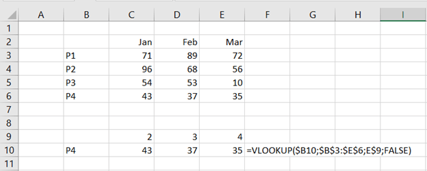
VLOOKUP consists of four arguments.
- Lookup value: which value to look after, in this case it is P4 in the cell B10.
- Table array: where to look after the look up value, B3:E6.
- Column index number: how many steps from B-column you have to take to enter the column where the look up value is, the B column is one. We need to take four steps to check the March values.
- Range lookup: are we looking after an exact match (false) or a rough match (true). I normally use false just like this time.
If you want that VLOOKUP returns an array, you can add an extra value on top of the return array, like C9 to E9.
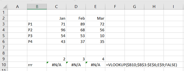
If the VLOOKUP does not find an exact match for the lookup value, the formula return #N/A.
This can be tackled with IF and ISERROR functions like:
=IF(ISERROR(VLOOKUP($B10;$B$3:$E$6;E$9;FALSE));”Not found”;(VLOOKUP($B10;$B$3:$E$6;E$9;FALSE)))
Now it is time to introduce our new friend XLOOKUP.
Now it is time to introduce our new friend XLOOKUP.
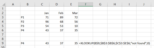
When you enter the formula, just activate the cell C9.
The arguments for XLOOKUP are:
- Lookup value: which value to look after, in this case it is P4 in the cell B9. This is similar to the VLOOKUP.
- Lookup array: list of values containing the lookup value, $B$3:$B$6.
- Return array: array of the values, in our case sales values, $C$3:$E$6.
- If not found: if the formula cannot return any value, the formula return this value. “not found.
- Match code: are we looking after an exact match or a rough match. I use 0 to have an exact match. This is same kind of as range lookup in VLOOKUP.
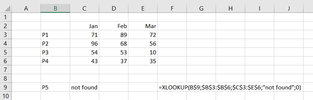
P5 cannot be found, so the result is “not found”.
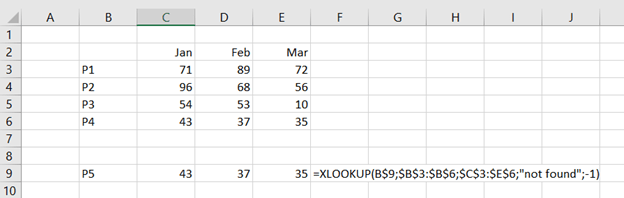
When match code is -1, the XLOOKUP returns next smaller value.

Another good thing with XLOOKUP is that it works also vertically, just like HLOOKUP.
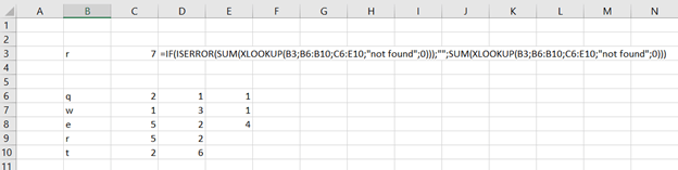
Another good thing with XLOOKUP is that as the function returns an array, you can frame with SUM function to get the sum of a row.
XLOOKUP returns an array which is advancement compared to VLOOKUP and HLOOKUP. XLOOKUP makes things easier.


