Data is downloaded from web. You should sum up the values you downloaded. However, this does not happen without some modification.

The numeric values don’t get summed.

The cell category is number.

Replacing the space with SUBSTITUTE does not work.

If you replace character number 160, then the thousand separator will disappear. SUM function does not work.

Again the cell category is number, but calculation does not work.

When you frame the previous sentence with VALUE function, the cell gets numeric category and calculation works fine.

=VALUE(SUBSTITUTE(B2;CHAR(160);””))

If you take value from cell with space, the VALUE function does not work.

This is an extension for my earlier OFFSET blog “Introducing OFFSET function”.

One application for OFFSET is selecting a value from a two dimensional report.

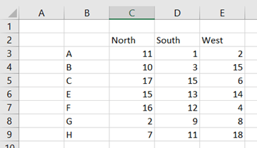
On the horizontal axis we have sales areas and products on vertical axis.

The issue is to enter sales area and product, and then receive the correct sales value.

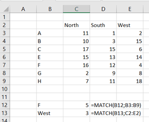
First we need to use MATCH function.

We have list of products in B3:B9. When we want to know what is the ordinal number of the given value. If we enter “F”, is it first, second, third or some other value in the B3:B9 ? The correct value is 5, as the “F” is 5^th letter in the range.

The same applies to the horizontal axis. “West” is the third value in the range C2:E2.

Like this.

Now, we can use OFFSET-function. We know, that F is 5^th and West 3^rd on axises.

In OFFSET-function, we need to first define the starting cell or reference, that is B2. Then we set how many steps we take vertically, that is five steps downwards, as we are looking for “F”. After that we decide step horizontally. We step three steps to right. As we are not expecting a range but a singe cell as the return value, height and width arguments are both 1.

The formula is  =OFFSET(B2;C12;C13;1;1) .

If you want to write the whole formula without interim values the formula goes like this:

=OFFSET(B2;MATCH(B12;B3:B9);MATCH(B13;C2:E2);1;1) .

Replace C12 with MATCH(B12;B3:B9) and

               B13 with MATCH(B13;C2:E2) .

As the OFFSET works with reference plus rows and columns, the examples above are not the only correct ones.

If you set reference as C3, you take one step down and one to right, instead of selecting B2 as the reference.

The OFFSET sentences are:

=OFFSET(C3;C12-1;C13-1;1;1) and

=OFFSET(C3;MATCH(B12;B3:B9)-1;MATCH(B13;C2:E2)-1;1;1) .