You bought a flat in 2010 for 130 k€ and sold it in 2020 for 185 k€. How many percent the value of the flat grew annually ?
The formula is ((start value /finish value)^(1/ start year/finish year))-1
This calculation is counting only full years, and calculation gives you a directional value. The idea is not to calculate exact value, but rather to give you an idea about magnitude.
The same value can be counted with own formula, if you feel that more convenient. The functions returns you a short message, if the function finds an error.
Function z_annual2(start_value, finish_value, start_year, finish_year)
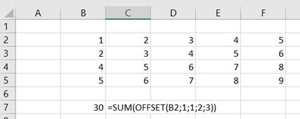
Reference. Where is the starting point of the formula ? In this example it is the cell B2.
Rows. How many steps the formula takes downwards from starting point. 1 means, the formula goes to B3.
Columns. How many steps the formula takes to the right from B3. One means, the formula ends up in C3.
Height: How high is the area starting from C3. Two means the area of C3:C4.
Width: How wide is area from C3:C4, three means area C3:E5.
SUM function returns the sum of area C3:E5.
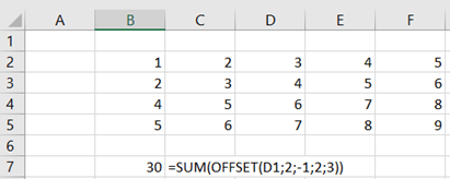
If you want to take steps upwards or to the left, enter negative values.
The same range C3:E5 can be defined in another way too.
To start with D1, you need to go two rows downwards and one column to the left.
=SUM(OFFSET(D1;2;-1;2;3))
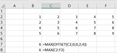
OFFSET can be framed with other function than SUM, for example MAX.
When the range is C2:F3, we can check what is the highest value in that range.
=MAX(OFFSET(C2;0;0;2;4))
On the other hand, you can count the same with direct MAX function.
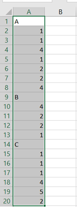
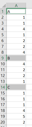
One application how to use OFFSET, is to count values for the sales report which is listing all the sales lines under the header. Range A10:A13 are the sales lines for the material B, valuing 9. The list is dynamic, there might a more a less values under the header.
The first thing is to pick up products which are letters. To pick up alphanumeric fields:
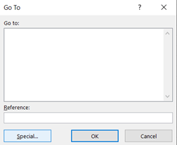
Activate the data area.
Select home – find & select – go to
Press special.
Select Constants radio button and unselect tick boxes apart from Text. Press ok.
Take control + C to copy letters.
Activate wanted destination cell and press control + V.
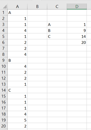
In order to find where does the area for A or B start, we need MATCH function.
The formula in D3 is =MATCH(C3;$A$1:$A$20). The formula returns the value 1, meaning A is the first cell in range A1:A20. B is 9th and C 14th. The last populated cell in column A has order number 20. The formula in the cell D6 is =COUNTA(A:A).
Now we can calculate the values between A and B.
The formula in D3 is =MATCH(C3;$A$1:$A$20).
From A1 to A20, what is the order number for “A”. That is one, meaning A is in the first cell in the range A1:20.
The formula for D4 is =MATCH(C4;$A$1:$A$20) and for D5 =MATCH(C5;$A$1:$A$20).
D6 shows how many populated cells there are in A-column. The formula is =COUNTA(A:A).
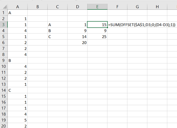
To the point, how to count sales volume for the product A.
The formula in E3 is =SUM(OFFSET($A$1;D3;0;(D4-D3);1)).
The OFFSET starts with the cell A1, that is with absolute reference. We take one step downwards, and no steps to right or left. The are starts in B1 and the area is eight steps of height and one of wide. That area is summed and the result is 15.
The second product B in E4 holds the formula =SUM(OFFSET($A$1;D4;0;(D5-D4);1)). The logic is same as earlier. A1 is the reference cell, then we take 9 steps downwards and zero steps horizontally. The area, to be summed, five steps of height and one step of width. The result is nine.