Weekday from WEEKDAY function

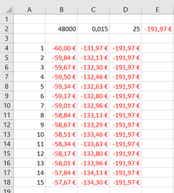
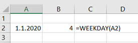
When you use WEEKDAY function in Excel, you enter a date like 1.1.2020 and maybe hope to see the weekday. However, WEEKDAY returns you a number. With Return_type argument, you can define the number, but number is still a number. It would be nice to have a weekday like Monday or Tuesday instead of the number.


I have seen some ways to have a weekday instead of number.

I like an IF-sentence.

=IF(WEEKDAY(A4)=1;”Sunday”;IF(WEEKDAY(A4)=2;”Monday”;IF(WEEKDAY(A4)=3;”Tuesday”;IF(WEEKDAY(A4)=4;”Wednesday”;IF(WEEKDAY(A4)=5;”Thursday”;IF(WEEKDAY(A4)=6;”Friday”;IF(WEEKDAY(A4)=7;”Saturday”)))))))

It is a bit long, but once I wrote it, you can just copy paste it.

Just paste the text to cell B4.

Another option is that you create your own function with the same logic.

Function z_wd(z_d As Date)

If WorksheetFunction.Weekday(z_d) = 1 Then

    z_wd = “Sunday”

ElseIf WorksheetFunction.Weekday(z_d) = 2 Then

    z_wd = “Monday”

ElseIf WorksheetFunction.Weekday(z_d) = 3 Then

    z_wd = “Tuesday”

ElseIf WorksheetFunction.Weekday(z_d) = 4 Then

    z_wd = “Wednesday”

ElseIf WorksheetFunction.Weekday(z_d) = 5 Then

    z_wd = “Thursday”

ElseIf WorksheetFunction.Weekday(z_d) = 6 Then

    z_wd = “Friday”

ElseIf WorksheetFunction.Weekday(z_d) = 7 Then

    z_wd = “Saturday”

End If

End Function

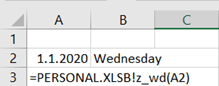
To use the function in B2 might be easier than direct IF-sentence.

Additional loan functions

In the previous blog, we checked basic loan functions.

If you pay a same payment for your loan every month, then one part of the payment is interest and another part payback of the loan.

To count how much of the payment is interest and how much payback, we will use IPMT and PPMT functions.

If we have a loan of 48 k, interest rate 1,5 % annually, and the payback period is 25 years. Then the monthly payment is around 192 €.

Now we would like to know how 192 € is divided between interest and loan payback.

The A column holds the periods meaning months. The B column includes the interest and C payback amounts. Column D equals to B plus C.

The formula in B4 is =IPMT($C$2/12;A4;$D$2*12;$B$2).

The formula in C4 is =PPMT($C$2/12;A4;$D$2*12;$B$2).

The arguments for the both formulas are:

  1. Rate. 1,5 % in C2 must be divided by 12 to get monthly value.
  2. Per. Which period is examined. In B4 we check the first period. The reference is relative, when you copy downwards, also the reference changes.
  3. Nper. Years needs to be multiplied by 12 to have number of months.
  4. Pv. Present value of the loan, amount of the loan is in B2.
  5. Fv. Future value, an optional argument.

For example, the first monthly payment of 191,97 € consists of 60 € interest and 131,97 € payback.

To check that the PPMT function works, copy the data down, that you will get all the 300 payments. Then sum up all the PPMTs, you should get 48 k.

As the IPMT and PPMT are to calculate one single period, cumulative interest or loan payback for several periods can be calculated with CUMIPMT and CUMPRINC.

To count how much interest and how much payback you pay during the first year, you can count that with IPMT and PPMT. Just sum B4:B15 and you will get 709,07 € for interest. Sum C4:C15 for payback amount, the result is 1594,57 €.

The same things can be counted with CUMIPMT and CUMPRINC.

The formulas are here for copy pasting:

=CUMIPMT(C2/12;D2*12;B2;1;12;0)

=CUMPRINC(C2/12;D2*12;B2;1;12;0)

The arguments for CUMIPMT and CUMPRINC are:

  1. Rate. Interest rate, we divide annual rate by 12 to get monthly rate.
  2. Nper. Number of payment periods, 25 years multiplied by 12 to have 300 months.
  3. Pv. Present value, amount of the loan taken 48 k.
  4. Start_period: From which period we are counting. In this case it is 1.
  5. End_period: The last period we are interested in. In this case it is 12.
  6. Type: Do the payment take place in the beginning or at the end of the period. We assume at the end.