We have a two dimensional table with unique axis.

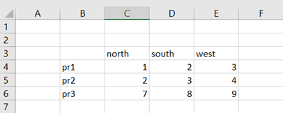
This example is simplified from real case. The user wants to know the value by entering values from both the axis. Like pr1 and south should return the value 2.

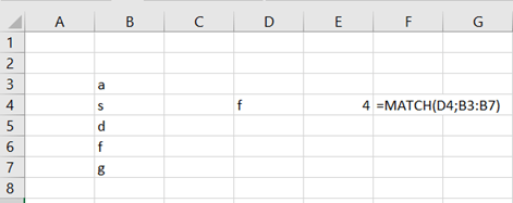
We need two formulas for this case, MATCH and INDEX. Both the formulas are relatively simple.

In the list f is the fourth letter.

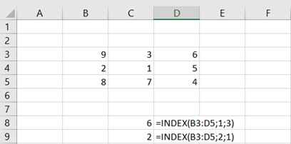
INDEX forms coordinates for the range.

Range(B3:D5) forms an array. B3 is a corner where you start counting row and columns. First row and third column is D3 and value 6. Second row and first column is B4, the value 2.

Entering values are in fields G2 and G3. The pr3 is searched in B4:B6 with MARCH, and west in C3:E3, also with MATCH. Then INDEX is using the values form MATCH functions to find out the value for pr3/west which equals to 9.

Both INDEX and MATCH are embedded in G8.

SUMPRODUCT is very versatile function. Only parameters you enter are multiple arrays. Therefore it can be used for multiple purposes in finance and accounting. I present here some examples, but there are much more.

The basic idea with SUMPRODUCT is multiply several arrays with each other.

Simply 3 * 1 = 3, 4 * 2 = 8 and 5 * 3 = 15. Sum of 3,8, and 15 equals to 26. You can end up with this result with SUMPRODUCT.

This blog is related to my earlier blog to count total debits and total credits. The same process is here done with SUMPRODUCT function.

In my example the total debits and credit have been counted with four different ways with SUMPRODUCT. Feel free, to find even more options to count the same process.

The content in cells C11:C14 is pasted here, so you can copy paste them, if needed.

=SUMPRODUCT($B$3:$M$8*($B$2:$M$2=C10))

=SUMPRODUCT(–($B$2:$M$2=C10)*$B$3:$M$8)

=SUMPRODUCT(–($B$3:$M$8)*($B$2:$M$2=C10))

=SUMPRODUCT(($B$2:$M$2=C10)*$B$3:$M$8)

All of these variations lead to the correct result. You need to define separately, range for debit and credit codes (B2:M2) and range for values (B3:M8). Please note, that arrays cannot be separated with semicolon but by multiplication sign.

One more additional use for SUMPRODUCT is to count total for account groups.

You have a list of income accounts. You want to count the total per account group. Like sum of accounts starting with 10. First array defines the values in range B3:B7, if two digits from left make up “10”. Sum range is D3:D7.

You can count the sum for account group with SUM and IF like this:

=SUM(IF(LEFT(B3:B7;2)=”10″;D3:D7))

Don’t forget control+shift+enter.

The debit and credit totals have the values vertically, account group total case horizontally. Still SUMPRODUCT tackles both the cases.

You have a list of income accounts. You want to count the total per account group. Like sum of accounts starting with 10. First array defines the values in range B3:B7, if two digits from left make up “10”. Sum range is D3:D7.

However, the criteria 10 needs to inside the formula not in a reference cell. Note also, that accounts values in B3:B7 are of text data type. The formula in G4 just does not work.