VBA

Searching for two terms

September 28, 2019 Ismo Heiskanen

Years ago I was asked, if it is possible to search with two search criterias in worksheet. So, I want to search both A and B whichever I find first. Normally you search in Excel with just one criteria like this:

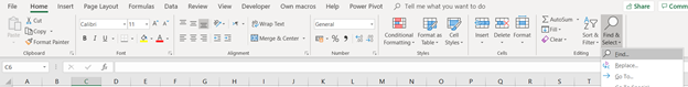
To find take home-find & select – find.

First search for A.

Then search for B.

If you however want to search for both A and B at the same go, then we need some further development.

Here is the VBA code from a recorded macro searching for A.

Sub Z_search()
‘
‘ Z_search Macro
‘

‘
Cells.Find(What:=”A”, After:=ActiveCell, LookIn:=xlFormulas, LookAt:= _
xlPart, SearchOrder:=xlByRows, SearchDirection:=xlNext, MatchCase:=False _
, SearchFormat:=False).Activate
End Sub

To modify the VBA, first the main block should be doubled that first the search term 1 is searched and the search term 2. Static “A” should be replaced by parameter. The main block is copied from recorded macro.

On Error Resume Next means that if VBA hits an error, the code is not stopped there. This is needed because if the macro does not find anything, it will face a run time error 91. With this line the VBA does not stop with run time error.

Here is the code

Sub z_search()
‘
‘ z_search Macro
‘

Dim s1, s2
s1 = InputBox(“1st search term”)
s2 = InputBox(“2nd search term”)

On Error Resume Next

‘ this part was recorded and then what-parameter was modified, I did not write this myself

Cells.Find(What:=s1, After:=ActiveCell, LookIn:=xlFormulas, LookAt:= _
xlPart, SearchOrder:=xlByRows, SearchDirection:=xlNext, MatchCase:=False _
, SearchFormat:=False).Activate

Cells.Find(What:=s2, After:=ActiveCell, LookIn:=xlFormulas, LookAt:= _
xlPart, SearchOrder:=xlByRows, SearchDirection:=xlNext, MatchCase:=False _
, SearchFormat:=False).Activate

End Sub

If the code find both the first term and the second term, then the program is showing the place of the second term, but this is a functionality.

Functions, VBA

Counting total debit or credit with SUM and SUMIF

September 17, 2019 Ismo Heiskanen

You have list of accounting postings. For some reason, you need to check that sum of debit postings equals to sum of credit postings. There might be an error in closing process, and you just want to double check in Excel that no mismatch has taken place in accounting. System should not allow a posting when debit differs from credit, but this is a case to really make sure that no mismatch exists.

Accounting data was simplified. Imagine, that you have hundreds of accounts and thousands of postings.

One simply option is to count with SUMIF. First, you need to count sum for every column like in row 10. Totals for debit and credit are counted with SUMIF. In SUMIF you need to first determine range for Ds and Cs that is B2:M2. Then criteria is needed whether it is D or C, B13 or B14. Finally you enter sum range B10:M10. If in row 2 the value equals to B13 or B14 then sum is counted from row 10. This works, but is you have lots of data, this might be bit difficult as you need to count each column sum separately.

Another bit easier solution is to count with SUMIF without interim SUMs. Write following formula =SUM(IF(B2:M2=B11;B3:M8)) in C11 and press control+shift+enter. The result should be {=SUM(IF(B2:M2=B12;B3:M8))}, but don’t write that, that is the outcome after control+shift+enter.

SUM is counted in M3:M8 if values in B2:M2 equals to B11. Don’t forget control+shift+enter.

Third option is to use column numbering.

COLUMN function is turning column letter to number.

In our case debits are in paired columns and credits in impaired.

Paired and impaired numbers can be traced by MOD function.

If MOD is 1 then the column is for debits and 0 for credits.

Row 10 includes sum of each row like M10 sums M3:M8. Row 9 determines whether the column number is paired or impaired. SUMIF in C12 is a normal SUMIF. First you need to feed the range meaning Ds and Cs, then criteria C or D is needed, last sum range is given.

Fourth option is based on paired and impaired column numbers. A custom made formula is summing up the values in paired or impaired columns. For paired cells dc parameter is 0 and impaired 1. Then activate the sum area. That’s all.

The custom made function:

Function z_dc(dc, rng As Range)

Dim cell As Range

Dim para

If dc = 0 Then

para = 0

ElseIf dc = 1 Then

para = 1

End If

z_dc = 0

For Each cell In rng

If (cell.Column) Mod 2 = para Then

z_dc = (z_dc + cell.Value)

End If

Next cell

End Function

Graphics

Combo chart

September 6, 2019 Ismo Heiskanen

Data here represents monthly values for parameter one. Required level for parameter one is five for H1 and six for H2. Data should be published graphically.

Activate the data and press line symbol under insert ribbon.

Select the first icon in the row.

Blue line values are parameter values and orange the requirement values.

Alternatively, you can select

The bar icon.

Select the first icon in the row.

Both data series, parameter and requirement, are shown as bars.

Maybe the best option would be a combination between the two chart types, bars and lines, like in two earlier examples. Parameter one would be bars and requirement a line. If the bar crosses the line, then the parameter is above the requirement. If the bar stays under the line, then the parameter has not met the criteria that month.

This can be selected in several ways in Excel.